Lecture 9: Bivariate relationship with NBA data

This is intended as an asynchronous, self-learning lecture.

Prep work

Self-learning task: run the following code to get a sense of the data and create two new variables (points per game, and categorized age)

library(Lock5Data)
library(tidyverse)
?NBAPlayers2024

# create new variables
NBAPlayers2024 <- NBAPlayers2024 %>%
  mutate(pointsPerGame = Points/Games) %>%
  mutate(age_cat = case_when(Age<=25 ~ 'Young',
                             Age<=30 & Age >25 ~ 'Middle',
                             Age >30 ~ 'Old'))

Bivariate relationship

Bivariate relationship refers to the relationship between TWO variables:

  • What graph/tool/statistics to use largely depends on the types of the two variables.

  • Description of the relationship is often open-ended and varies based on the context of the data.

  • Always remember that Correlation does not imply causation!

Self-learning task: use an AI agent, type in the following prompt: Provide five examples of “correlation does not imply causation”; some examples should include numeric variables and some should include categorical variables.

Numeric + Numeric

Correlation coefficient

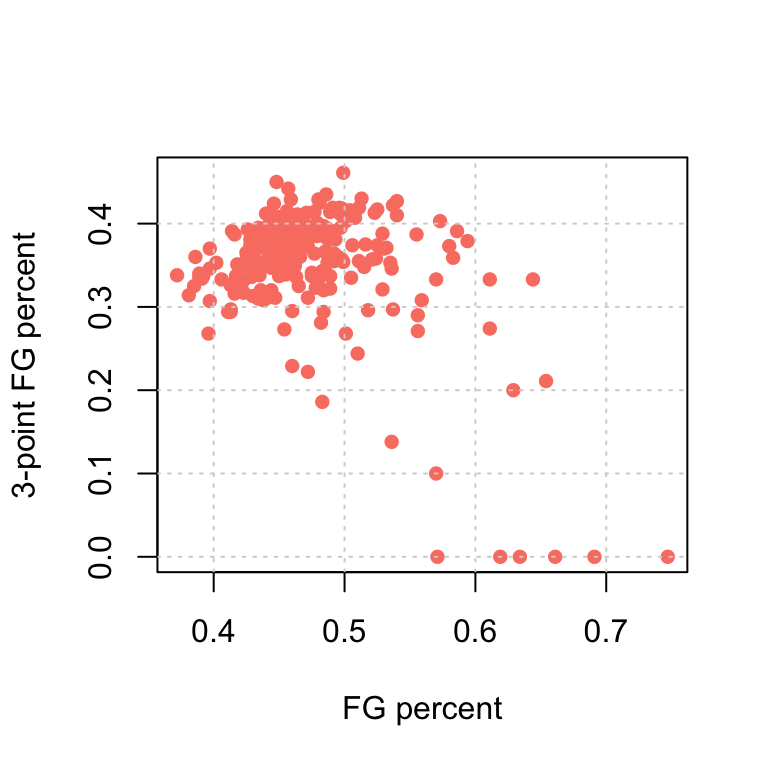
Example question: is there a relationship between FGPct and FG3Pct for players in the dataset?

  • Use (Pearson) correlation coefficient for two numeric (scale) variables
[1] NA

We get an NA as there are NA values for both of the variables; to remedy:

cor(NBAPlayers2024$FGPct,NBAPlayers2024$FG3Pct,use="pairwise.complete.obs")
[1] -0.4493933
  • Self-learning task: Run ?cor() to bring up the help page; you can see that it is easy to specify what to do with NA values and the type of correlation coefficient to calculate with the cor() function

  • A correlation coefficient close to 0 signals weak to no linear relationship between the two variables; a correlation coefficient close to 1 or -1 signals strong linear relationship

Interpretation for a positive correlation (\(>> 0.1\))

Self-learning task: Find a variable positively correlated with FGPct and write an interpretation.

Click to see an example solution

Players with a higher field goal percentage tend to have a higher numbers of rebound, on average

[1] 0.5886253

Interpretation for a negative correlation (\(<< -0.1\)):

Self-learning task: Write an interpretation for the correlation between FGPct and FG3Pct we found above.

Click to see an example solution

Players with a higher field goal percentage tend to have a lower three-point field goal percentage, on average.

  • Avoid causal language: you should not write “The higher the field goal percentage, the lower the three-point field goal percentage”; or “As the field goal percentage increases, the three-point field goal percentage decreases” as this kind of language implies a causal relationship.

Inferential statistics

We have been working with many different data and can describe the data in many ways (summary statistics, visualizations, correlations, etc.). However, data does NOT equal to the truth!

  • In any survey data (like the Changing Childhood Project): respondents are only a random sample of the population. If we see that, for instance, 23% of respondents from the United States are optimistic, it does not mean that exactly 23% of the entire U.S. population are optimistic.

  • In the NBA example: a player’s true ability (of shooting field goals, for instance) is a latent variable that cannot be directly measured. For instance, if in the 2024 NBA season, player 1 has a higher field goal percentage than player 2, it doesn’t necessarily mean that player 1 is better than player 2; maybe he is just lucky (i.e., his success is “due to random chance”).

  • Another way to think about this: most of the time, data is not reproducible: if I conduct the same survey again with different respondents, I will get different answers and different statistics; if NBA player 1 is better than player 2 in 2024, it is not a guarantee that he will also be better in 2025.

p-value and statistical significance

  • Descriptive statistics, also referred to as Exploratary Data Analysis (EDA), is about describing the data

  • Inferential statistics is about generalizing the conclusion to the entire population and/or the truth

  • Typically, a “hypothesis test” is conducted and a p-value is obtained

    • If p-value is large (>0.05): the conclusion is not significant and due to random chance

    • If p-value is small (<0.05): the conclusion is statistically significant

  • What is the conclusion in this case?

    Click to see answer

    Players with a higher field goal percentage tend to have a lower three-point field goal percentage, on average. The correlation is statistically significant and not likely due to random chance (p-value \(< 0.001\)).


    Pearson's product-moment correlation

data:  NBAPlayers2024$FG3Pct and NBAPlayers2024$FGPct
t = -7.6292, df = 230, p-value = 6.224e-13
alternative hypothesis: true correlation is not equal to 0
95 percent confidence interval:
 -0.5465566 -0.3402912
sample estimates:
       cor 
-0.4493933 

Scatterplot

Recall, a scatterplot is a bivariate graph that visualizes the relationship between two numeric/scale variables.

Self-learning task: Generate the following graph with both base R function and ggplot.
Click to see solution
# base R
plot(x=NBAPlayers2024$FGPct,
     y=NBAPlayers2024$FG3Pct,
     xlab='FG percent',
     ylab='3-point FG percent',
     pch=16,
     col='salmon')
grid()

# ggplot
NBAPlayers2024 %>% ggplot(aes(x=FGPct, y=FG3Pct)) +
  labs(x='FG percent',y='3-point FG percent') +
  geom_point(color='salmon') +
  theme_bw()

Numeric + Categorical

Summary by group

Example question: Is there a relationship between FGPct and the position of the player (Pos)?

  • In this case, we are comparing FGPct of players in different positions. The variable Pos is the grouping variable (i.e., “factor”). We already know how to do this!

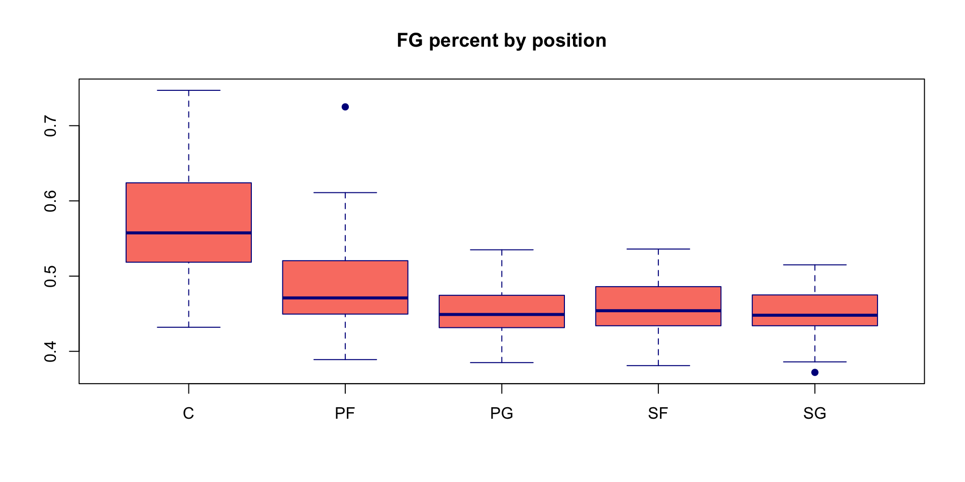
Self-learning task: Use R to obtain the following information and generate the graph.

Pos mean(FGPct) median(FGPct) min(FGPct) max(FGPct)
C 0.5664444 0.5575 0.432 0.747
PF 0.4862115 0.4710 0.389 0.725
PG 0.4511628 0.4490 0.385 0.535
SF 0.4553962 0.4540 0.381 0.536
SG 0.4527736 0.4480 0.372 0.515
Click to see solution
NBAPlayers2024 %>% 
  group_by(Pos) %>%
  summarise(mean(FGPct),median(FGPct),min(FGPct),max(FGPct))

boxplot(NBAPlayers2024$FGPct ~ NBAPlayers2024$Pos,
        border='darkblue',
        col='salmon',
        pch=16,
        xlab=NA,
        ylab=NA, 
        main='FG percent by position')

Statistical significance

We see that FGPct differ by position for NBA players in the 2024 season. For instance, Centers have a much higher field goal percentage, on average. But is this difference due to random chance? In other words, does FGPct differ significantly by position, on average? This can be answered using a model called “ANOVA.” You don’t need to know the details of this model, but you should be able to interpret a given p-value. In this case, p-value is essentially 0 (\(2\times10^{-16}\)), so we can conclude that FGPct DOES differ significantly by position.

                    Df Sum Sq Mean Sq F value Pr(>F)    
NBAPlayers2024$Pos   4 0.3769 0.09422   42.21 <2e-16 ***
Residuals          232 0.5178 0.00223                   
---
Signif. codes:  0 '***' 0.001 '**' 0.01 '*' 0.05 '.' 0.1 ' ' 1

Self-learning task: Does the average FGPct differ significantly between point guards and power forwards? The following R code conducts an “independent samples t-test.” Report the p-value and write a conclusion.

t.test(NBAPlayers2024$FGPct[NBAPlayers2024$Pos=='PG'],
       NBAPlayers2024$FGPct[NBAPlayers2024$Pos=='PF'])

    Welch Two Sample t-test

data:  NBAPlayers2024$FGPct[NBAPlayers2024$Pos == "PG"] and NBAPlayers2024$FGPct[NBAPlayers2024$Pos == "PF"]
t = -3.7172, df = 81.391, p-value = 0.0003685
alternative hypothesis: true difference in means is not equal to 0
95 percent confidence interval:
 -0.05380784 -0.01628966
sample estimates:
mean of x mean of y 
0.4511628 0.4862115 
Click to see solution

The average FGPct DOES differ significantly between point guards and power forwards (p-value \(= 0.0003685\))

Categorical + categorical

Contingency table

  • Is there a relationship between age_cat and position?
  • A contingency table shows the count breakdown between these two categorical variables
    
     Middle Old Young
  C      13   7    16
  PF     18  10    24
  PG     11  12    20
  SF     20   8    25
  SG     18   4    31
  • Counts are typically not as useful as percentages. There are different ways to calculate percentages based on the denominator.
    
     Middle   Old Young
  C   0.055 0.030 0.068
  PF  0.076 0.042 0.101
  PG  0.046 0.051 0.084
  SF  0.084 0.034 0.105
  SG  0.076 0.017 0.131

This table shows that, out of all players, 5.5% are Centers and “young”. This table is not that useful to determine the relationship between position and age.

    
     Middle   Old Young
  C   0.361 0.194 0.444
  PF  0.346 0.192 0.462
  PG  0.256 0.279 0.465
  SF  0.377 0.151 0.472
  SG  0.340 0.075 0.585

Here, we can say that there may be a relationship. For instance, among small forwards, 55.6% are “young,” whereas among shooting guards, 35.3% are “young.” Statistical significance can be determined using a “Fisher’s exact test” or a “chi-square test.”


    Pearson's Chi-squared test

data:  mytable
X-squared = 8.5431, df = 8, p-value = 0.3823

Since the p-value is 0.3823, there is NO significant relationship between position and age categories.