Lecture 5: data visualization
Data: the changing childhood project by UNICEF
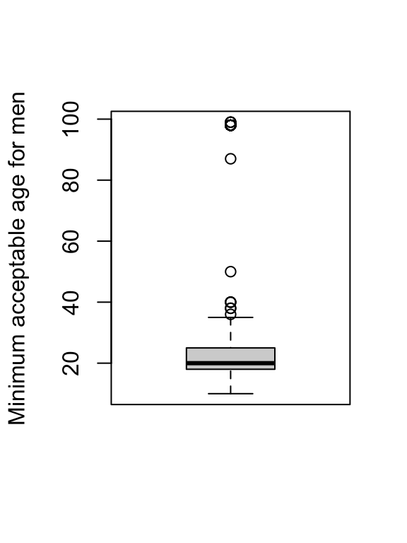
Boxplot
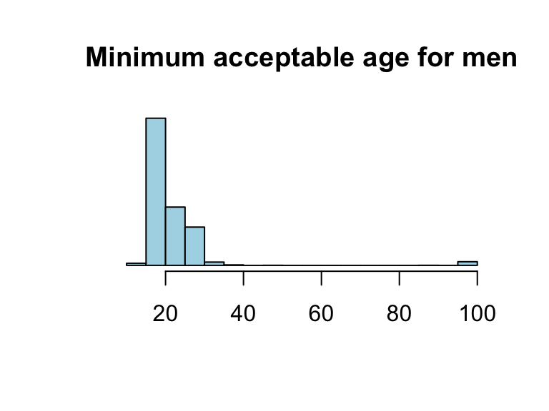
Histogram
- In base R, visualization elements can be modified by adding arguments within the function
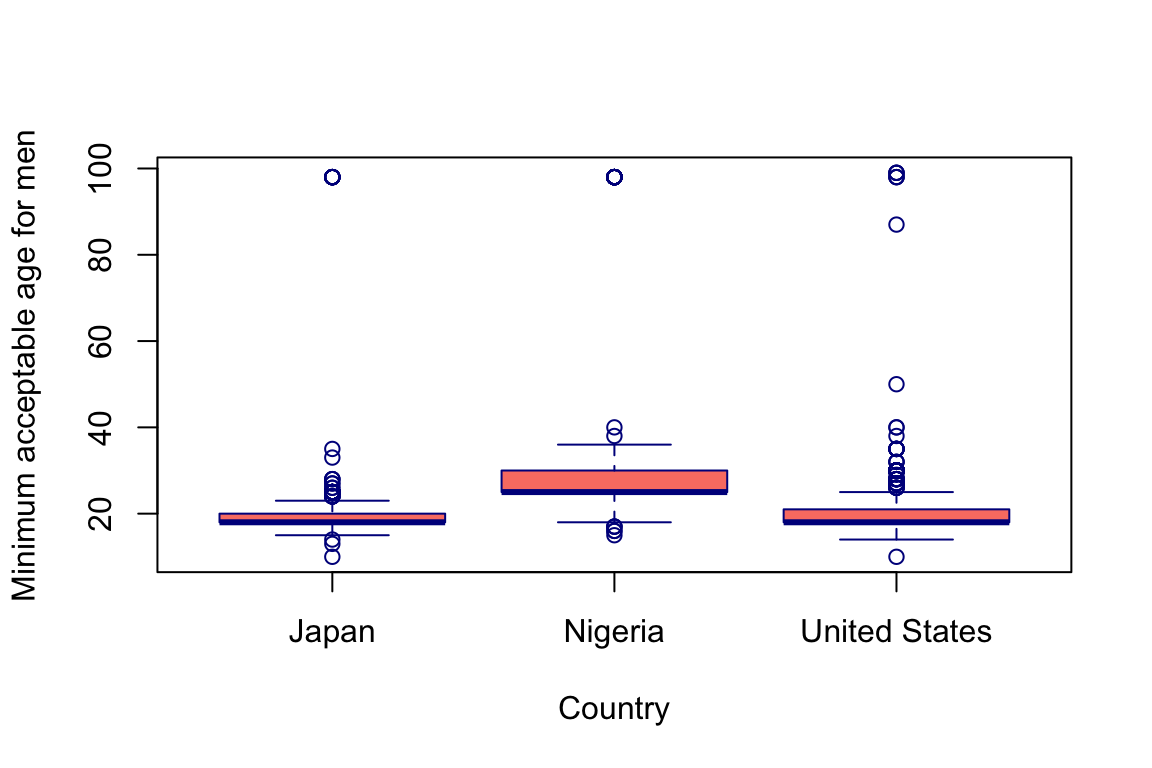
Side-by-side boxplots
Scatterplot
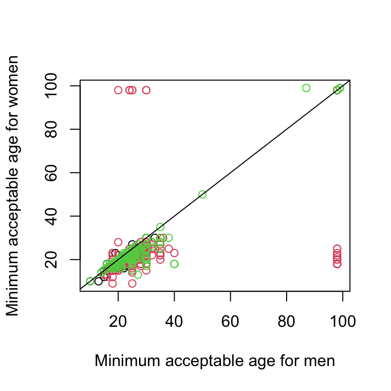
Comment: with base R, plotting can be fast, but it’s not very easy to incooperate other steps (like removing invalid values 97, 98, 99). Adding layers (e.g., a reference line) is also not very convenient.
Example 1
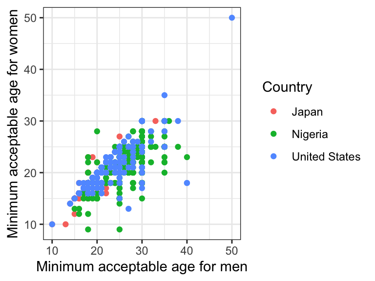
Example 2
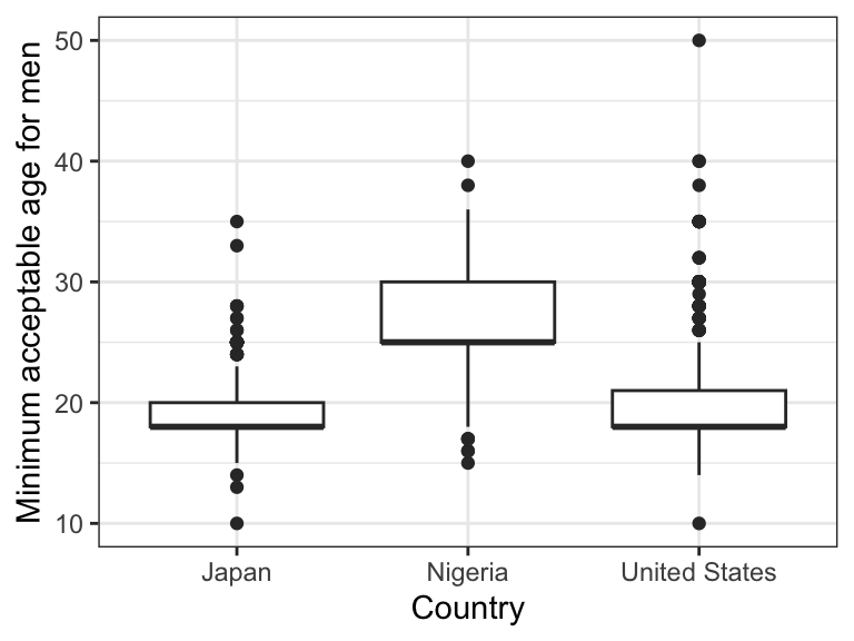
Example 1 explained
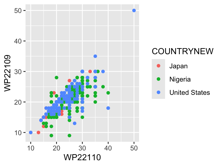
Example 2 explained
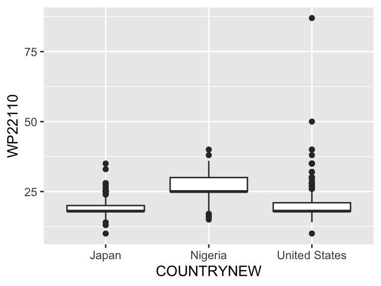
geom_violin
Use the same code for example 2, but change geom_boxplot to geom_violin.
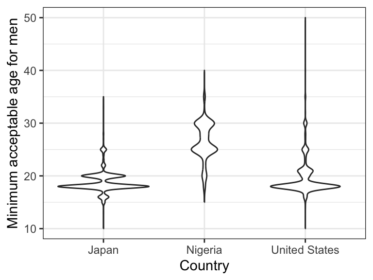
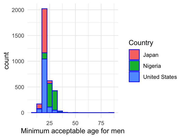
geom_histogram
- Recall: histogram is univariate; y-axis is always frequency, so we don’t need a y=_ mapping
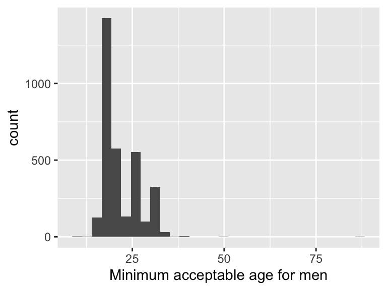
- Add arguments in geoms
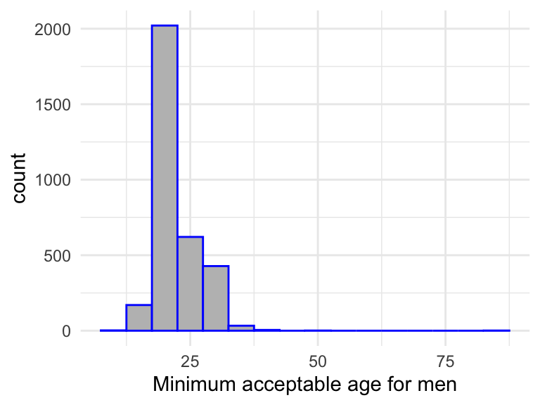
- Note the differences in the syntax convention:
- base R col vs ggplot fill
- base R border vs ggplot color
- esp. “color” (ggplot) vs “col” (base R)
- Add another dimension (i.e., map another variable to another aesthetic)
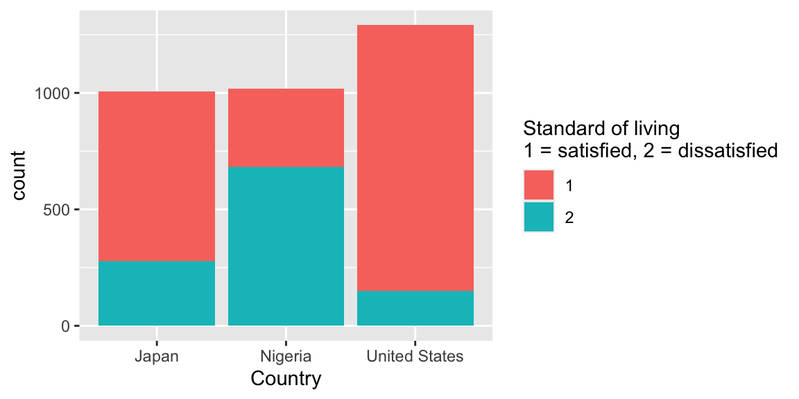
geom_bar
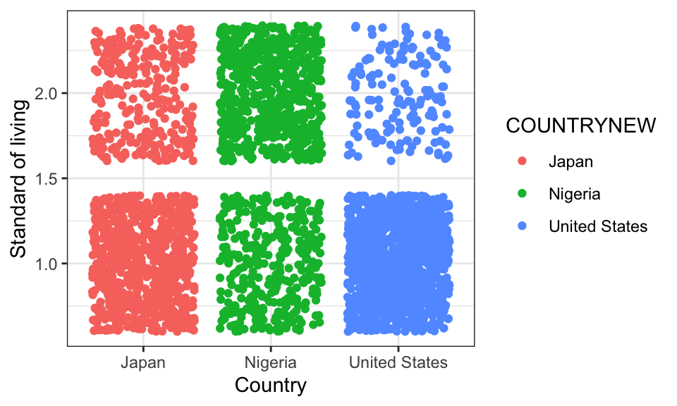
geom_jitter
Scatterplots can be hard to read when both variables are categorical. Jitter separates overlapping responses.
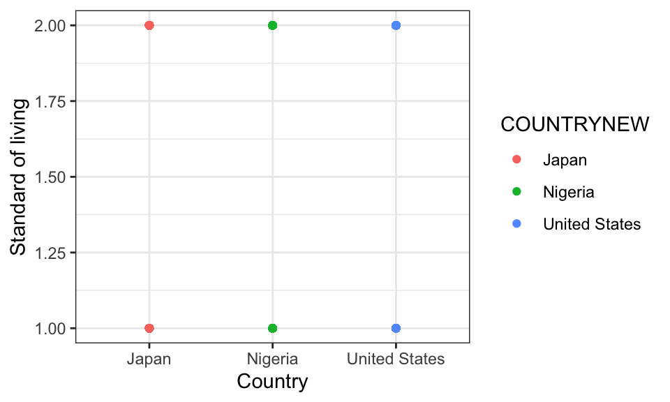
Change geom_point() to geom_jitter()
geom_text
df.child.small %>%
  filter(WP22110 < 97, WP22109 < 97) %>%
  group_by(COUNTRYNEW) %>%
  summarise(mean_male_age=mean(WP22110),
            mean_female_age=mean(WP22109),
            .groups="drop") %>%
  ggplot(aes(x=mean_female_age, y=mean_male_age, label=COUNTRYNEW)) +
  geom_text(size=0.5) +
  labs(x="mean min age for women", y="mean min age for men")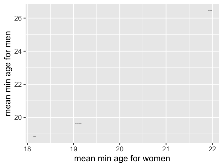
- Try: change geom_text to geom_label
- Try: add geom_point
Comment: it is very easy to combine data manipulation steps with ggplot.
Customize ggplot with +
ggplot offers a very convenient syntax (+) to add elements and layers
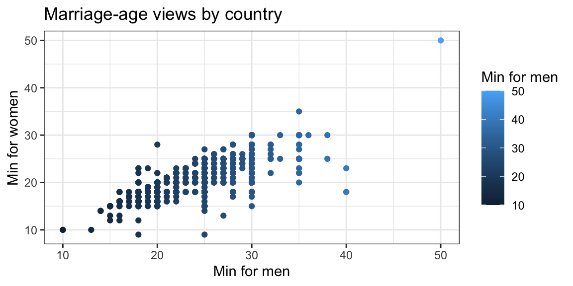
Comment: in this example, the same variable (WP22110) is mapped to both the x-axis and the color aesthetic. This is not recommended as it is redundant.
Example: change gradient color
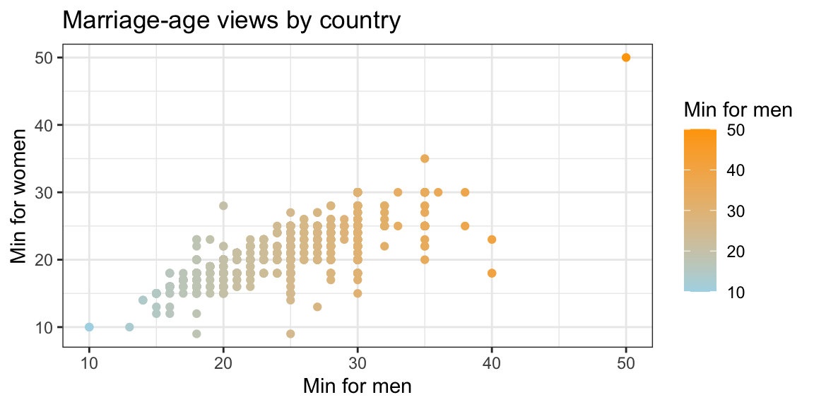
Example: change categorical color
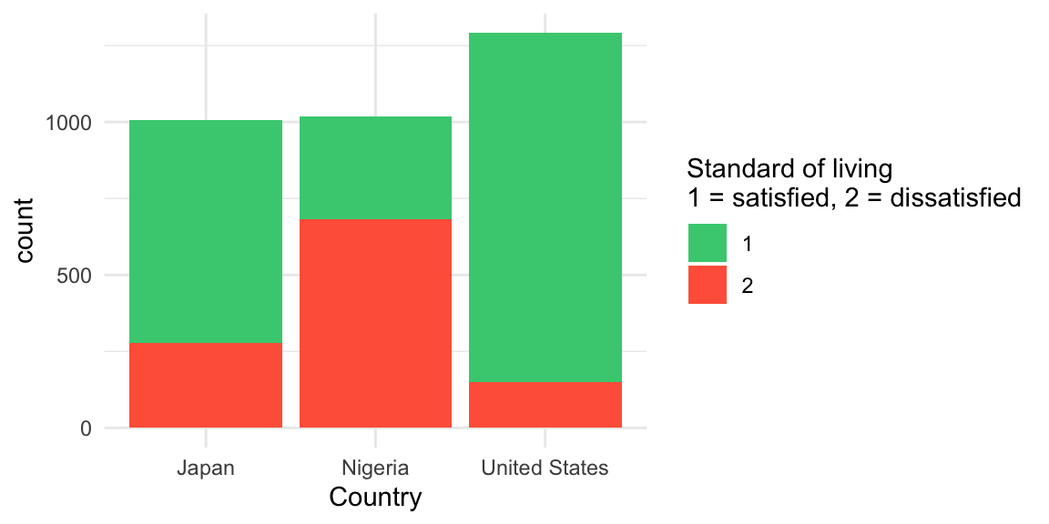
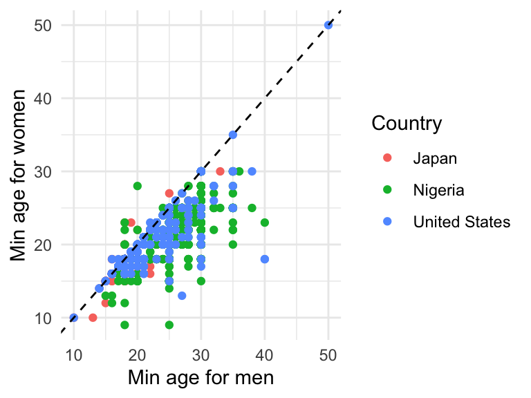
Example: add a line
Example: multiple panels by a grouping variable
WP22091 records whether respondents identify most with their city or area (1), their country (2), or the world (3). WP30 records satisfaction with standard of living: satisfied (1) or dissatisfied (2).
df.child %>%
  filter(COUNTRYNEW %in% c("Germany", "United States"),
         WP22091 %in% 1:3, WP30 %in% 1:2) %>%
  ggplot(aes(x = as.factor(WP22091), y = as.factor(WP30))) +
  geom_jitter() +
  theme_bw() +
  facet_wrap(~COUNTRYNEW) +
  ggtitle("Identity and standard-of-living satisfaction") +
  labs(
    x = "Identity (1 = city/area, 2 = country, 3 = world)",
    y = "Standard of living (1 = satisfied, 2 = dissatisfied)"
  )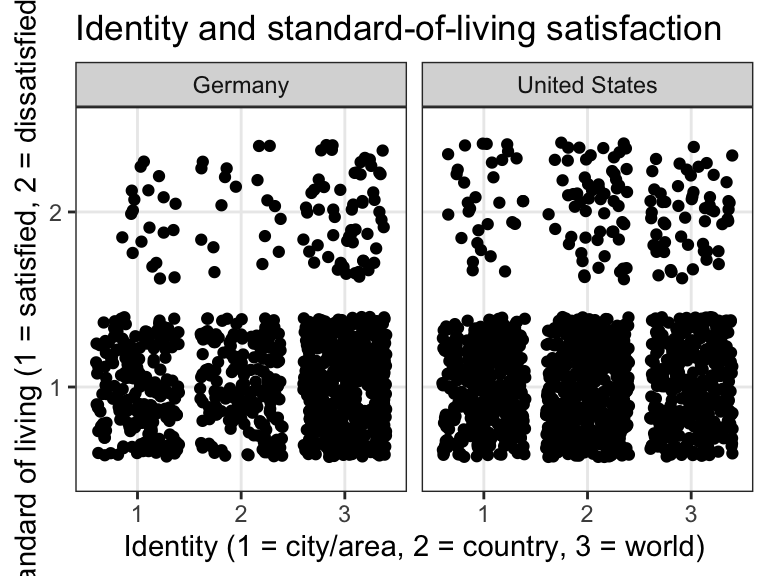
Comment: ggplot works very well with tidyverse functions; as you can see in this example, we actually do not need to use the smaller dataset, since it’s easy to filter information from the large dataset before visualization.
Exercise
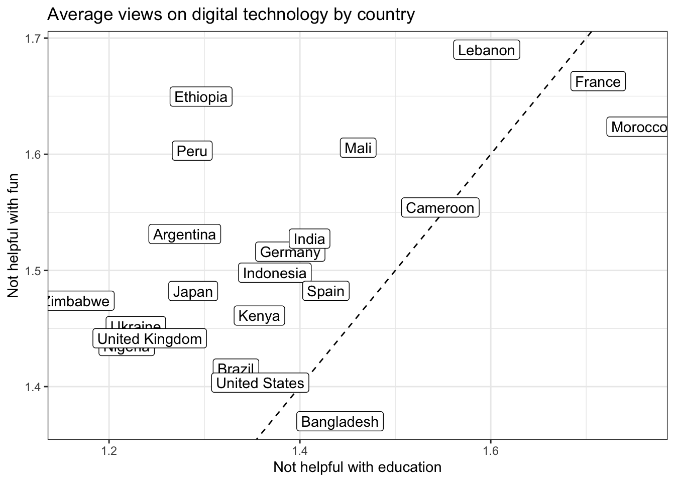
WP22071: whether digital technology helps children with education.WP22072: whether digital technology helps children have fun.- For both questions,
1= a lot,2= a little, and3= not at all. Other response codes are excluded.
Try to reproduce the following graph. You can also use other variables of your interest (refer to the codebook).
Show code
df.child %>%
  filter(WP22071 %in% 1:3, WP22072 %in% 1:3) %>%
  group_by(COUNTRYNEW) %>%
  summarise(
    mean_education = mean(WP22071),
    mean_fun = mean(WP22072),
    .groups = "drop"
  ) %>%
  ggplot(aes(x = mean_education, y = mean_fun, label = COUNTRYNEW)) +
  geom_abline(slope=1, intercept=0, linetype="dashed") +
  geom_label() +
  theme_bw() +
  labs(
    title = "Average views on digital technology by country",
    x = "Not helpful with education",
    y = "Not helpful with fun"
  )