Lecture 3: Univariate distributions

Data: NBA players

Prep work

library(Lock5Data)
library(tidyverse)
?NBAPlayers2024
#data("NBAPlayers2024") # optional
#data() # gives a list of available dataset
NBAPlayers2024$pointsPerGame <-
  NBAPlayers2024$Points/NBAPlayers2024$Games

Univariate distribution: location, spread, and shape

Overview

  • To describe a univariate distribution, we focus on three important properties: location, spread, and shape

  • Tools: statistics, tables, and visualizations

    • A statistic is a numeric summary of data (e.g.: sample mean is a statistic; sample maximum is a statistic)
  • Important statistics:

    • Mean, median, mode
    • Percentiles
    • Min, max
    • Range and Interquartile Range (IQR)
    • Standard deviation and variance

Location: mean, median, mode

  • Location (also referred to as central tendency) is a measure of a typical/average value

  • Example: what is the mean, median, and mode for this data?

sleep <- c(5,5,6,6,6,7,7,7,8,14)
  • For numeric variables, use mean and/or median
    • Example: typically, how many hours do students sleep?
    • Median is more robust to outliers
    • When mean and median values are very different, it signals very skewed distribution and the existence of outliers
  • In R (note, there is no built-in function for mode):
summary(sleep)
   Min. 1st Qu.  Median    Mean 3rd Qu.    Max. 
    5.0     6.0     6.5     7.1     7.0    14.0 
mean(sleep)
[1] 7.1
median(sleep)
[1] 6.5
table(sleep) # table () gives frequency for numeric variables
sleep
 5  6  7  8 14 
 2  3  3  1  1 
summary(as.factor(sleep)) # summary() gives frequency for factor variables
 5  6  7  8 14 
 2  3  3  1  1 
# equivalent code with pipe operator
sleep |> as.factor() |> summary()
 5  6  7  8 14 
 2  3  3  1  1 
  • Q: how can you convert the frequency to percentages?
  • Q: how do you use R to automatically give you the mode?
Show code
table(sleep) %>% 
  as.data.frame() %>%
  mutate(Percent = Freq / sum(Freq)) %>%
  arrange(desc(Freq))
  sleep Freq Percent
1     6    3     0.3
2     7    3     0.3
3     5    2     0.2
4     8    1     0.1
5    14    1     0.1
  • For categorical variables (i.e., factor), use mode
    • Example: based on mtcars, what kind of transmission type (0=automatic,1=manual) do cars typically have?
table(mtcars$am)

 0  1 
19 13 

Percentiles

  • The percentile (rank) of a value is the percentage below that value

  • The kth percentile of a variable is a value such that k percent are below that value

  • Special percentiles: first, second and third quartiles (i.e., Q1, Q2, and Q3) correspond to the 25th, 50th, and 75th percentiles; Q2 is the median

  • Percentiles (especially Q1, Q2, and Q3) provide a sense of the location of the distribution
summary(NBAPlayers2024$pointsPerGame)
   Min. 1st Qu.  Median    Mean 3rd Qu.    Max. 
  4.273   9.769  13.375  14.442  19.085  34.692 
quantile(NBAPlayers2024$pointsPerGame, c(0.95, 0.75, 0.05))
      95%       75%        5% 
26.032767 19.084507  6.121994 

Spread: range and IQR

  • Spread can be measured by range and interquartile range (IQR)

    • range: min to max
    • IQR: Q1 to Q3 (i.e., range for the middle 50% of people)
summary(NBAPlayers2024$FG3Pct)
   Min. 1st Qu.  Median    Mean 3rd Qu.    Max.     NAs 
 0.0000  0.3360  0.3640  0.3501  0.3910  0.4610       5 
range(NBAPlayers2024$FG3Pct,na.rm = T)
[1] 0.000 0.461
summary(NBAPlayers2024$FGPct)
   Min. 1st Qu.  Median    Mean 3rd Qu.    Max. 
 0.3720  0.4400  0.4620  0.4777  0.4980  0.7470 
quantile(NBAPlayers2024$FGPct, c(0.25, 0.75), na.rm = T)
  25%   75% 
0.440 0.498 
IQR(NBAPlayers2024$FGPct, na.rm = T)
[1] 0.058
  • Are NBA players more consistent in their field goal shooting ability, or in 3-point field goal shooting ability?

  • Range is very affected by outliers!

Boxplot

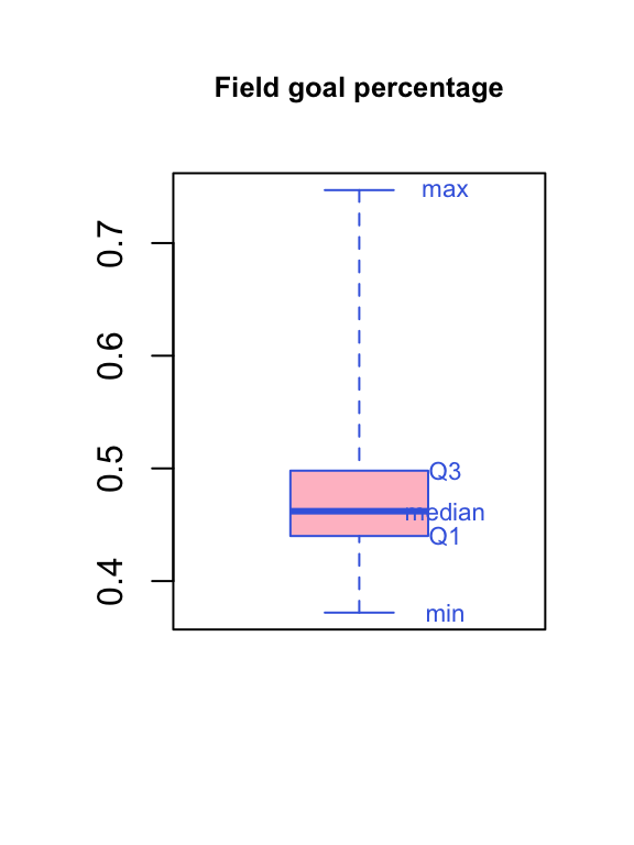
Boxplot is based on only five numbers: min, Q1, Q2, Q3, max (also called the five-number summary)

Show code
boxplot(NBAPlayers2024$FGPct,
        main=paste('Field goal percentage'),
        col='pink',
        border='royalblue',
        cex.main=0.8,range=0)

# `text()` adds text to an *existing* plot at the specified coordinate
text(1.25,quantile(NBAPlayers2024$FGPct,na.rm = T),
     labels=c('min','Q1','median','Q3','max'),
     col='royalblue',
     cex=0.7)
Spread: standard deviation (SD) and variance

  • SD is a measure of how spread out the data points are (“average distance of each data point to the mean”)
  • SD has the same unit as the data
GPA <- c(3.2,3.3,3.4)
sd(GPA)  #small SD, consistent GPA
[1] 0.1
TEMP <- c(50,60,90,100)
mean(TEMP); sd(TEMP) #large SD, lots of variation in temp
[1] 75
[1] 23.80476
  • Variance is the square of SD
var(GPA)
[1] 0.01

Shape: histogram and skewness

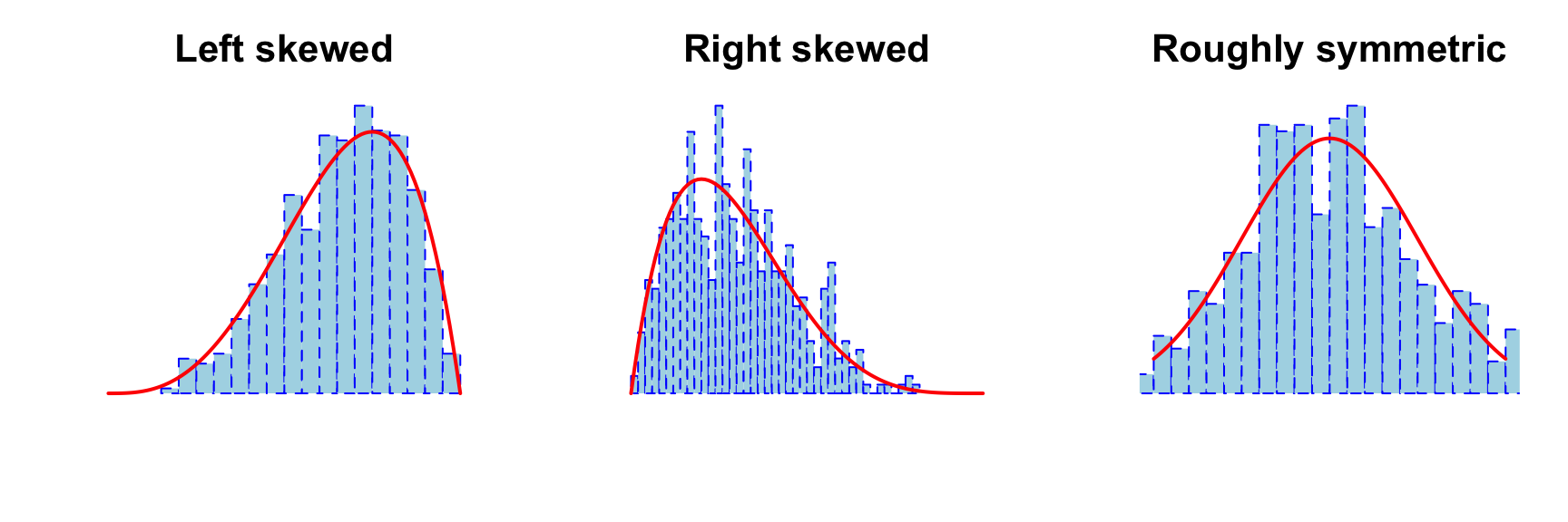
  • For determining the direction of skewness, look for tail values; extreme tail values are referred to as outliers

    • If tail values or extreme values are LARGE: right skewed (positive skew); e.g., income, house price, etc.
    • If tail values or extreme values are SMALL: left skewed (negative skew); e.g., age at death, retirement age, etc.
  • Histogram is a widely used univariate plot (in base R, use hist())

  • When describing shape, pay attention to: skewness, outliers, number of modes, and any other unusual pattern in the data
Exercise 1

Give a thorough description of the variable FGPct (Field goal percent), using statistics and visualizations as needed. Mention properties of location and spread, and describe the shape of the distribution.

Show solution

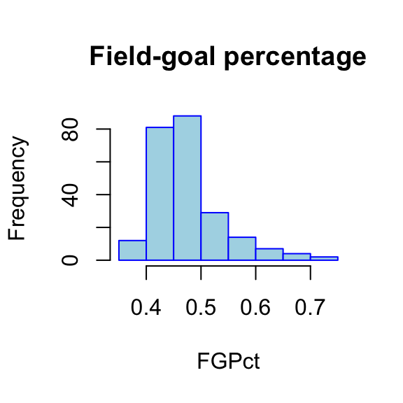
The field-goal percentages based on NBA data from 2024 range from 0.372 to 0.747. The mean is 0.478, while the median is 0.462, so a typical player has a field-goal percentage of about 46%. The middle 50% of players have field-goal percentages from 0.440 to 0.498, giving an interquartile range of 0.058. The standard deviation is 0.062.

The distribution is right-skewed: the mean is higher than the median, and the upper tail extends farther than the lower tail.

range(NBAPlayers2024$FGPct, na.rm = TRUE)
[1] 0.372 0.747
mean(NBAPlayers2024$FGPct, na.rm = TRUE)
[1] 0.4776709
median(NBAPlayers2024$FGPct, na.rm = TRUE)
[1] 0.462
quantile(NBAPlayers2024$FGPct, c(0.25, 0.75), na.rm = TRUE)
  25%   75% 
0.440 0.498 
IQR(NBAPlayers2024$FGPct, na.rm = TRUE)
[1] 0.058
sd(NBAPlayers2024$FGPct, na.rm = TRUE)
[1] 0.06157083
hist(NBAPlayers2024$FGPct, main = "Field-goal percentage", xlab = "FGPct", col = "lightblue", border = "blue")

Z-score

Z-score

  • Z-score (or standardized score) of a variable is calculated as (value - mean) / sd

  • It’s used to standardize a variable so that you can make sense of the value regardless of the scale or unit

  • Example: Tom has an SAT of 1400. Jerry has an ACT of 28. Who has a better score? We know that:

    • SAT: mean=1100, sd=150
    • ACT: mean=25, sd=2
  • Q: what’s the z-score for Tom? for Jerry?

  • Q: Interpretations of the z-scores?

Show solution

Tom’s z-score is \((1400 - 1100) / 150 = 2\). Jerry’s z-score is \((28 - 25) / 2 = 1.5\).

Tom’s SAT score is 2 standard deviations above the SAT mean, while Jerry’s ACT score is 1.5 standard deviations above the ACT mean. Relative to their respective tests, Tom has the higher score.

in R:

# by hand: a vector is created
a <- NBAPlayers2024$FGPct
z1 <- (a - mean(a))/sd(a)

# using scale(): a matrix is created
z2 <- scale(NBAPlayers2024$FGPct)

Exercise 2

  1. Calculate the z-scores of FGPct and FG3Pct and store the z-scores as separate variables in the data frame.

  2. Print the information for Stephen Curry and give an interpretation for the z-scores of FGPct and FG3Pct. Relatively speaking, is he better at field goals or 3-point field goals?

  3. Find a player whose field goal percentage is above the average, but 3-point field goal percentage is below the average.

  4. Find a player who is very capable in both field goal and 3-point field goal.

  5. What is the mean and sd for the z-scores of FGPct and FG3Pct?

Show solution
NBAPlayers2024 <- NBAPlayers2024 %>%
  mutate(FGPct.z = as.numeric(scale(FGPct)),
         FG3Pct.z = as.numeric(scale(FG3Pct)))

NBAPlayers2024 %>%
  filter(Player == "Stephen Curry") %>%
  select(Player, Team, FGPct, FG3Pct, FGPct.z, FG3Pct.z)

NBAPlayers2024 %>%
  filter(FGPct.z > 0, FG3Pct.z < 0) %>%
  select(Player, Team, FGPct, FG3Pct, FGPct.z, FG3Pct.z,MinPerGame)%>%
  arrange(desc(MinPerGame))

NBAPlayers2024 %>%
  filter(FGPct.z > 1, FG3Pct.z > 1) %>%
  select(Player, Team, FGPct, FG3Pct, FGPct.z, FG3Pct.z)

summary(NBAPlayers2024$FGPct.z)
summary(NBAPlayers2024$FG3Pct.z)
  1. Add the standardized variables with scale(), as shown in the code above.

  2. Stephen Curry’s FGPct z-score is -0.449, while his FG3Pct z-score is 0.768. His field-goal percentage is about 0.449 standard deviations BELOW the sample mean, while his 3-point percentage is 0.768 standard deviations ABOVE the sample mean. Relative to other players, he is stronger at 3-point field goals.

  3. DeMar DeRozan is one example: his FGPct is 0.038 SDs above the mean, while his FG3Pct is 0.226 SDs below the mean.

  4. Jalen Williams is one example of a player who is very capable in both areas: his FGPct z-score is 1.012 and his FG3Pct z-score is 1.020, so both are more than one standard deviation above their respective means.

  5. The mean of each z-score variable is approximately 0, and the standard deviation is 1; this is expected by how z-scores are calculated.