Lecture 2: Data types

Data: Tallest building

Exercise: tallest buildings

  • Go to the Wikipedia page on List of Tallest Buildings
  • We will only look at the top 10 tallest buildings
    1. Create a vector that stores the Height (m) of the top 10 tallest buildings
    2. Use R to verify that the vector you created has a length of 10
    3. Calculate the average Height in meters
    4. Convert height from meters to ft and store it in a new vector
    5. Print the values of the new vector and check that these values are the same as Height (ft) given in Wikipedia
    6. Create corresponding vectors for the number of floors and year built for the top 10 tallest buildings
    7. Create a vector of {0, 1} values, where 0 means the building was built in 2015 or before, and 1 means otherwise
    8. Generate a scatterplot of Floors by Height (m), set the color to “col=year_ind+2,” where “year_ind” is the indicator vector created in the last step
Show solution

Prep work

Import a dataset

Download the dataset “tallest building_2026.csv”

You need to specify the location (file path) of your dataset when you export or import a dataset. For simplicity:

# Put the data (.csv) in the same folder as the code (.R)
df.building <- read.csv(file='tallest building_2026.csv')

# OR #
df.building <- read.csv(file.choose())

In general:

  • Use “/” and Tab to navigate through folders
  • Use “../” to go up to the parent folder
  • If you want to check your current folder, use getwd() (“get working directory”)
  • To export a CSV file, use write.table()

In addition, load necessary packages

library(tidyverse)

Types of data

  • Basic types: numeric, double, logical, character, integer
  • Use typeof() or class() to check
class(df.building$Height_m)
[1] "numeric"
typeof(df.building$Height_m)
[1] "double"
class(df.building$Floors)
[1] "character"
class(df.building$Year > 2010)
[1] "logical"
  • Use functions of the form as.XXX() to switch between different types
df.building$Year > 2010
as.numeric(df.building$Year > 2010)
# entries in a vector are always of the same type
a <- c(1, 2, T, 'red'); a
[1] "1"    "2"    "TRUE" "red" 
class(a)
[1] "character"

Data modification

  • Issue 1: Height_f is a character vector (not numeric) because it contains commas. We need to get rid of the commas before converting it to numeric
class(df.building$Height_f)
[1] "character"
# Does not work: need to get rid of comma
as.numeric(df.building$Height_f)
 [1] NA NA NA NA NA NA NA NA NA NA NA NA NA NA NA NA NA NA NA NA NA NA NA NA NA
[26] NA NA NA NA NA NA NA NA NA NA NA NA NA NA NA NA NA NA NA NA NA NA NA NA NA
[51] NA NA NA NA NA NA NA NA NA NA NA NA NA NA NA NA NA NA NA NA NA NA NA NA NA
[76] NA NA NA NA NA NA NA NA NA NA NA NA NA NA NA NA NA NA NA NA NA NA NA
# Get rid of comma
gsub(pattern = ',', 
     replacement = '',
     df.building$Height_f)
 [1] "2717" "2227" "2073" "1972" "1966" "1819" "1776" "1740" "1740" "1731"
[11] "1667" "1614" "1588" "1560" "1550" "1516" "1513" "1503" "1488" "1483"
[21] "1483" "1483" "1480" "1480" "1454" "1450" "1449" "1439" "1428" "1404"
[31] "1401" "1397" "1394" "1388" "1388" "1386" "1380" "1367" "1356" "1354"
[41] "1352" "1350" "1342" "1321" "1316" "1292" "1289" "1288" "1287" "1280"
[51] "1274" "1273" "1270" "1263" "1260" "1257" "1256" "1251" "1251" "1250"
[61] "1248" "1237" "1234" "1232" "1232" "1227" "1226" "1225" "1215" "1210"
[71] "1210" "1210" "1208" "1205" "1200" "1191" "1180" "1180" "1178" "1177"
[81] "1175" "1175" "1169" "1168" "1168" "1168" "1166" "1166" "1163" "1163"
[91] "1163" "1162" "1155" "1155" "1153" "1150" "1149" "1148"
# Putting things together
df.building$Height_f <- 
  as.numeric(gsub(pattern = ',', replacement = '', df.building$Height_f))

# Equivalent code with pipe operator
df.building$Height_f <- df.building$Height_f %>% 
  gsub(pattern = ',', replacement = '') %>%
  as.numeric()
  • Issue 2: Take a look at the Floors variable. This format is difficult to work with. To parse a text using R, you need to be very specific about the text pattern. This is done using “regular expression” (a pattern language used to search, match, and manipulate text).
df.building$Floors 
 [1] "163 (+ 2 below ground)" "118 (+ 5 below ground)" "128 (+ 5 below ground)"
 [4] "120 (+ 3 below ground)" "115 (+ 5 below ground)" "123 (+ 6 below ground)"
 [7] "104 (+ 5 below ground)" "111 (+ 5 below ground)" "97 (+ 4 below ground)" 
[10] "109 (+ 8 below ground)" "101 (+ 5 below ground)" "101 (+ 3 below ground)"
[13] "108 (+ 4 below ground)" "101 (+ 6 below ground)" "98 (+ 4 below ground)" 
[16] "87 (+ 3 below ground)"  "81 (+ 3 below ground)"  "98 (+ 4 below ground)" 
[19] "95 (+ 6 below ground)"  "94 (+ 5 below ground)"  "88 (+ 5 below ground)" 
[22] "88 (+ 5 below ground)"  "89 (+ 5 below ground)"  "95 (+ 5 below ground)" 
[25] "88 (+ 4 below ground)"  "108 (+ 3 below ground)" "98 (+ 4 below ground)" 
[28] "101 (+ 4 below ground)" "84 (+ 2 below ground)"  "88 (+ 4 below ground)" 
[31] "62 (+ 4 below ground)"  "85 (+ 3 below ground)"  "101 (+ 6 below ground)"
[34] "98 (+ 2 below ground)"  "60"                     "85 (+ 3 below ground)" 
[37] "88 (+ 3 below ground)"  "88"                     "101 (+ 6 below ground)"
[40] "80 (+ 3 below ground)"  "88 (+ 6 below ground)"  "101 (+ 5 below ground)"
[43] "80"                     "86 (+ 3 below ground)"  "79 (+ 5 below ground)" 
[46] "77 (+ 2 below ground)"  "77"                     "68 (+ 5 below ground)" 
[49] "88 (+ 4 below ground)"  "80 (+ 2 below ground)"  "70 (+ 7 below ground)" 
[52] "80 (+ 3 below ground)"  "73 (+ 1 below ground)"  "72 (+ 4 below ground)" 
[55] "69 (+ 3 below ground)"  "80 (+ 4 below ground)"  "75 (+ 6 below ground)" 
[58] "82 (+ 4 below ground)"  "88 (+ 5 below ground)"  "102 (+ 1 below ground)"
[61] "87 (+ 4 below ground)"  "81"                     "73 (+ 3 below ground)" 
[64] "60 (+ 5 below ground)"  "70 (+ 4 below ground)"  "78 (+ 3 below ground)" 
[67] "93 (+ 4 below ground)"  "77 (+ 5 below ground)"  "86 (+ 7 below ground)" 
[70] "70"                     "73 (+ 3 below ground)"  "73 (+ 6 below ground)" 
[73] "77 (+ 4 below ground)"  "72 (+ 4 below ground)"  "55 (+ 3 below ground)" 
[76] "101 (+ 5 below ground)" "68 (+ 5 below ground)"  "62 (+ 3 below ground)" 
[79] "80"                     "65 (+ 5 below ground)"  "77 (+ 3 below ground)" 
[82] "94"                     "75 (+ 2 below ground)"  "71 (+ 5 below ground)" 
[85] "71 (+ 5 below ground)"  "79"                     "82 (+ 2 below ground)" 
[88] "82 (+ 2 below ground)"  "54"                     "79 (+ 3 below ground)" 
[91] "74 (+ 3 below ground)"  "90 (+ 2 below ground)"  "59"                    
[94] "86 (+ 4 below ground)"  "106"                    "68 (+ 4 below ground)" 
[97] "60 (+ 6 below ground)"  "75 (+ 4 below ground)" 
df.building <- df.building %>%
  mutate(
    Floors_num = str_extract(Floors, "^\\d+") %>% 
      as.integer(),
    Floors_additional = str_extract(Floors, "(?<=\\(\\+ )\\d+") %>% 
      as.integer(),
    Floors_additional_text = str_extract(Floors, "(?<=\\d )[^(]+(?=\\))") %>% 
      str_trim()
    )

# double check
str(df.building)
'data.frame':   98 obs. of  12 variables:
 $ Rank                  : int  1 2 3 4 5 6 7 8 8 10 ...
 $ Name                  : chr  "Burj Khalifa" "Merdeka 118" "Shanghai Tower" "Mecca Royal Clock Tower" ...
 $ Height_m              : num  828 679 632 601 599 ...
 $ Height_f              : num  2717 2227 2073 1972 1966 ...
 $ Floors                : chr  "163 (+ 2 below ground)" "118 (+ 5 below ground)" "128 (+ 5 below ground)" "120 (+ 3 below ground)" ...
 $ City                  : chr  "Dubai" "Kuala Lumpur" "Shanghai" "Mecca" ...
 $ Location              : chr  "United Arab Emirates" "Malaysia" "China" "Saudi Arabia" ...
 $ Year                  : int  2010 2024 2015 2012 2017 2017 2014 2016 2019 2018 ...
 $ Comments              : chr  "Tallest building in the world since 2009" "Tallest building in Southeast Asia" "Tallest building in East Asia, tallest twisted building in the world; contains the highest luxury hotel in the world" "Tallest building in Saudi Arabia, tallest clock tower and contains the highest museum in the world" ...
 $ Floors_num            : int  163 118 128 120 115 123 104 111 97 109 ...
 $ Floors_additional     : int  2 5 5 3 5 6 5 5 4 8 ...
 $ Floors_additional_text: chr  "below ground" "below ground" "below ground" "below ground" ...

Factors

Factors

  • Location is entered as character (i.e., text) data
class(df.building$Location)
[1] "character"
unique(df.building$Location)
 [1] "United Arab Emirates" "Malaysia"             "China"               
 [4] "Saudi Arabia"         "South Korea"          "United States"       
 [7] "Taiwan"               "Hong Kong"            "Russia"              
[10] "Vietnam"              "Kuwait"               "Egypt"               
[13] "Indonesia"            "Turkey"               "Canada"              
  • We might want to treat it as a factor instead
df.building$Location_F <- as.factor(df.building$Location)
  • Key difference: factors can be treated as numbers but characters cannot
as.numeric(df.building$Location_F)
 [1] 13  7  2  9  2 10 14  2  2  2 11  2  4  2 14  8 15  2  7  2  7  7  2  2  2
[26] 14  2  2 14  2 14 14 13 14 14  2  2  2 13  6  4 10  2  2  2  3  2  2 13  2
[51]  2  2 14  9  2  2  5  2 13 14 13 13  2  2  2  4  8  2  2  2 13  2  2  4 14
[76] 14 13  2  2  2  2 13 13  2  2 13 13 13 13  2  2  8 12 13  1  2  2  2
as.numeric(df.building$Location)
 [1] NA NA NA NA NA NA NA NA NA NA NA NA NA NA NA NA NA NA NA NA NA NA NA NA NA
[26] NA NA NA NA NA NA NA NA NA NA NA NA NA NA NA NA NA NA NA NA NA NA NA NA NA
[51] NA NA NA NA NA NA NA NA NA NA NA NA NA NA NA NA NA NA NA NA NA NA NA NA NA
[76] NA NA NA NA NA NA NA NA NA NA NA NA NA NA NA NA NA NA NA NA NA NA NA

Useful functions for factors

unique(df.building$Location_F)
 [1] United Arab Emirates Malaysia             China               
 [4] Saudi Arabia         South Korea          United States       
 [7] Taiwan               Hong Kong            Russia              
[10] Vietnam              Kuwait               Egypt               
[13] Indonesia            Turkey               Canada              
15 Levels: Canada China Egypt Hong Kong Indonesia Kuwait Malaysia ... Vietnam
levels(df.building$Location_F)
 [1] "Canada"               "China"                "Egypt"               
 [4] "Hong Kong"            "Indonesia"            "Kuwait"              
 [7] "Malaysia"             "Russia"               "Saudi Arabia"        
[10] "South Korea"          "Taiwan"               "Turkey"              
[13] "United Arab Emirates" "United States"        "Vietnam"             
  • Factors are often used as a grouping variable. tapply() allows you to analyze data by groups.
tapply(df.building$Year,df.building$Location_F,median)
              Canada                China                Egypt 
              2026.0               2019.0               2023.0 
           Hong Kong            Indonesia               Kuwait 
              1997.5               2022.0               2011.0 
            Malaysia               Russia         Saudi Arabia 
              2008.5               2016.0               2016.5 
         South Korea               Taiwan               Turkey 
              2018.0               2004.0               2024.0 
United Arab Emirates        United States              Vietnam 
              2012.5               2017.0               2018.0 
tapply(df.building$Height_m,df.building$Location_F,mean)
              Canada                China                Egypt 
            351.4000             412.6417             393.8000 
           Hong Kong            Indonesia               Kuwait 
            409.3250             382.9000             412.6000 
            Malaysia               Russia         Saudi Arabia 
            509.0750             396.6333             493.0000 
         South Korea               Taiwan               Turkey 
            483.0500             508.0000             352.0000 
United Arab Emirates        United States              Vietnam 
            400.9500             423.9000             461.2000 
# OR #
df.building %>%
  group_by(Location_F) %>%
  summarise(median(Year), mean(Height_m), length(Year))
# A tibble: 15 × 4
   Location_F           `median(Year)` `mean(Height_m)` `length(Year)`
   <fct>                         <dbl>            <dbl>          <int>
 1 Canada                        2026              351.              1
 2 China                         2019              413.             48
 3 Egypt                         2023              394.              1
 4 Hong Kong                     1998.             409.              4
 5 Indonesia                     2022              383.              1
 6 Kuwait                        2011              413.              1
 7 Malaysia                      2008.             509.              4
 8 Russia                        2016              397.              3
 9 Saudi Arabia                  2016.             493               2
10 South Korea                   2018              483.              2
11 Taiwan                        2004              508               1
12 Turkey                        2024              352               1
13 United Arab Emirates          2012.             401.             16
14 United States                 2017              424.             12
15 Vietnam                       2018              461.              1
  • Plotting with Location as a character vector is not easy
plot(df.building$Location,df.building$Height_m) #error!
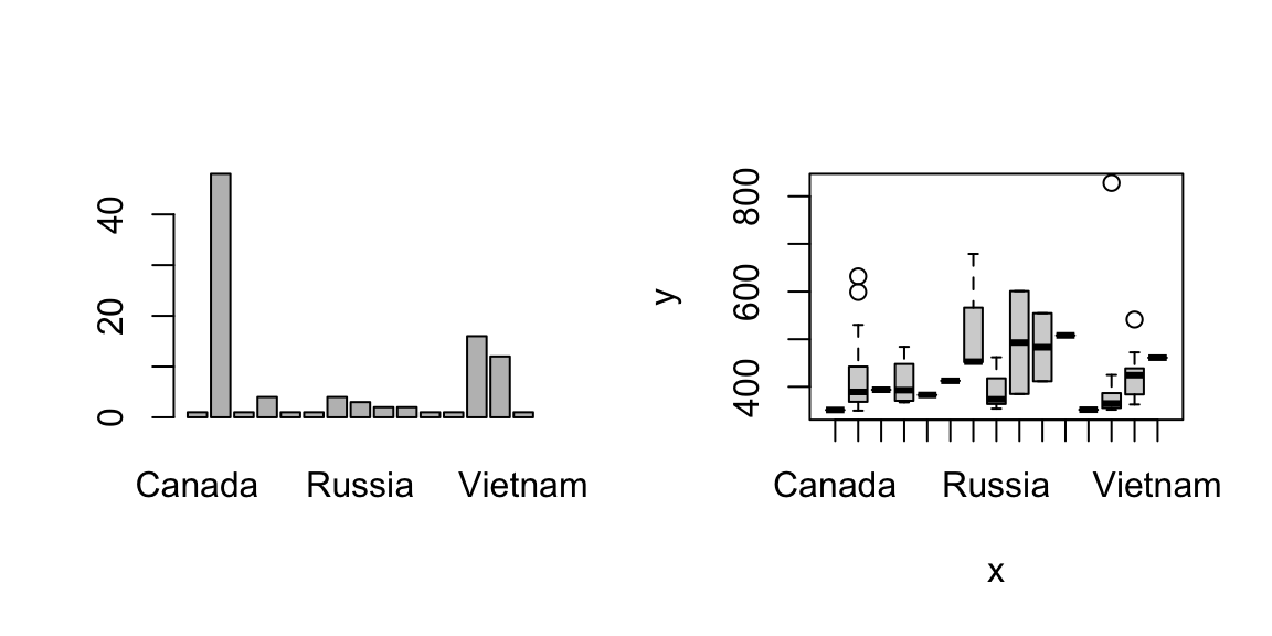
  • Plotting with Location_F:
par(mfrow=c(1,2))
plot(df.building$Location_F) #bar graph
plot(df.building$Location_F,df.building$Height_m)  #boxplots by Location

From vector to data: data frames

Data frame

In most cases, datasets in R are stored as a data frame

  • Subsetting requires two indices (row, column)
df.building[1,2] # first row, second column
[1] "Burj Khalifa"
  • Easier: each component in a data frame corresponds to a column (i.e., a variable); use $ to get the component
df.building$Name[1] # name of first building

Useful functions

names(df.building) # variable names
dim(df.building) # dimension (row, column)
nrow(df.building) # number of rows
str(df.building) # summary information
head(df.building) # first few rows
tail(df.building) # last few rows

Exercise: data frame basics

  • Print out the names of the first 5 buildings

  • Calculate the average height in meters of the first 5 buildings (should get 667.8)

  • Create a new vector, ft.per.floor, by height (ft) / number of floors

To add a variable to an existing data frame

df.building$ft.per.floor <- ft.per.floor
# OR 
df.building['ft.per.floor'] <- ft.per.floor
  • Calculate the average ft.per.floor of buildings by Location

  • Create a scatterplot of year by height (ft), colored by Location (hint: use the factor version)

Show solution
df.building$Name[1:5]
[1] "Burj Khalifa"            "Merdeka 118"            
[3] "Shanghai Tower"          "Mecca Royal Clock Tower"
[5] "Ping An Finance Centre" 
df.building$Height_m[1:5] %>% mean()
[1] 667.8
df.building$ft.per.floor <- df.building$Height_f/df.building$Floors_num

tapply(df.building$ft.per.floor, df.building$Location_F, mean)
              Canada                China                Egypt 
            10.87736             16.39246             16.77922 
           Hong Kong            Indonesia               Kuwait 
            15.63356             16.74667             16.92500 
            Malaysia               Russia         Saudi Arabia 
            17.06015             14.50640             16.98750 
         South Korea               Taiwan               Turkey 
            14.07748             16.50495             19.57627 
United Arab Emirates        United States              Vietnam 
            15.15999             16.90919             18.67901 
df.building %>% 
  group_by(Location_F) %>% 
  summarise(mean(ft.per.floor))
# A tibble: 15 × 2
   Location_F           `mean(ft.per.floor)`
   <fct>                               <dbl>
 1 Canada                               10.9
 2 China                                16.4
 3 Egypt                                16.8
 4 Hong Kong                            15.6
 5 Indonesia                            16.7
 6 Kuwait                               16.9
 7 Malaysia                             17.1
 8 Russia                               14.5
 9 Saudi Arabia                         17.0
10 South Korea                          14.1
11 Taiwan                               16.5
12 Turkey                               19.6
13 United Arab Emirates                 15.2
14 United States                        16.9
15 Vietnam                              18.7
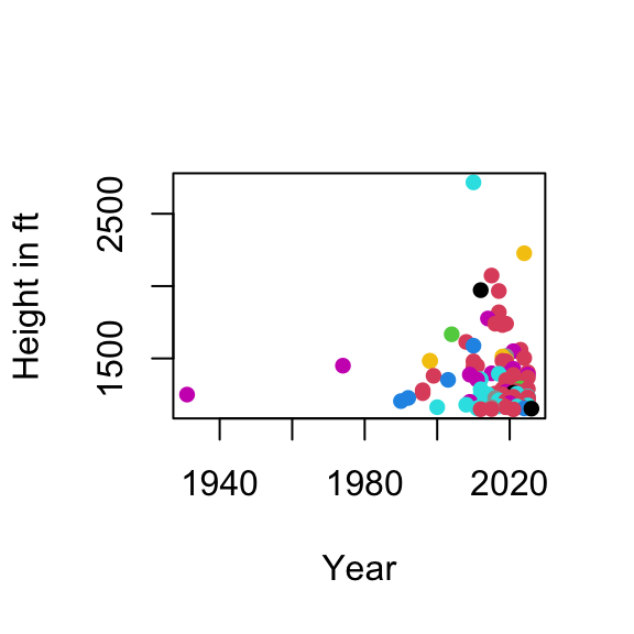
plot(df.building$Year,
     df.building$Height_f, 
     col = df.building$Location_F,
     xlab='Year',
     ylab='Height in ft',
     pch=16)

Matrix

Matrix

df.building.matrix <- as.matrix(df.building)
class(df.building.matrix)
[1] "matrix" "array" 
  • $ doesn’t work for getting variables from a matrix
  • Subsetting can be done using square brackets: matrix[row, column]
  • Variable names are now column names
colnames(df.building.matrix)
dim(df.building.matrix) 
df.building.matrix[1,3] #first row, third column
df.building.matrix[1,] #information for the first row
df.building.matrix[,2] #information for the second column
  • All entries in df.building.matrix are converted to characters
  • This is because entries in a matrix must have the same type
  • Matrices are more useful for storing only numeric values
  • In comparison: recall that a data frame allows variables to have different types

A more general R object: list

List

  • Suppose we also want to store these information
sample.size <- nrow(df.building)
variables <- names(df.building)
  • We have the following R objects
    1. df.building: a 61 x 9 data frame
    2. sample.size: a numeric value
    3. variables: a character vector of size 9
  • Q: What if we want to store all three objects in one R object?

List

  • A: Create a list with three components
list.building <- list(data=df.building,
               sample.size=sample.size,
               variables=variables)
  • Note: if a name is not provided for a component, it will be indexed by number
  • List is very general: each component can be of different length or type
  • Use $ to extract any component
  • Try list.building$... to print out each component to double-check
  • Another way to extract component: square bracket
    • list.building["COMPONENT"] is identical to list.building$COMPONENT
  • Benefit of using $: no need to spell; use Tab
  • Benefit of using [","]: can return more than one component in a more automated fashion
TORETURN <- c('variables', 'sample.size')
list.building[TORETURN]
$variables
 [1] "Rank"                   "Name"                   "Height_m"              
 [4] "Height_f"               "Floors"                 "City"                  
 [7] "Location"               "Year"                   "Comments"              
[10] "Floors_num"             "Floors_additional"      "Floors_additional_text"
[13] "Location_F"             "ft.per.floor"          

$sample.size
[1] 98

Useful functions for lists

Handling a list is very similar to handling a data frame

length(list.building) # number of components
names(list.building) # names of the components
str(list.building) # summary information

# add new component
list.building$mean_height <- mean(list.building$data$Height_m)

You can combine lists with c(); for instance: c(list.building, newlist)

R functions

R functions

  • R functions follow the same pattern: function_name(argument1 = XXX, argument2 = XXX, ...)
plot(df.building$Height_m,df.building$Floors_num) #shorter version
plot(x=df.building$Height_m,y=df.building$Floors_num) #full version
  • Use ?function_name to bring up the help menu

pipe operator (tidyverse package)

The pipe operator, %>%, is a different syntax for calling R functions: FUNCTION(x) is the same as x %>% FUNCTION

In recent R versions, you can also use |> as the pipe operator (no package required); it has slightly different behavior than %>% (will be discussed when the differences come up)

vec <- c(1, 1, 5)
mean(vec)
vec %>% mean()  # can omit the parentheses
vec |> mean() # must have the parentheses

For functions with multiple arguments: by default, R recognizes the argument being piped as the first argument; or you can use “.” or “_” as a placeholder to specify which argument is being piped

# these code are equivalent
plot(df.building$Height_m,df.building$Floors_num,xlab='Height')

df.building$Height_m %>% 
  plot(df.building$Floors_num,xlab='Height')

df.building$Height_m %>% 
  plot(x=., y=df.building$Floors_num,xlab='Height')

df.building$Height_m |>
  plot(x=_, y=df.building$Floors_num,xlab='Height') 

Exercise: scatterplot

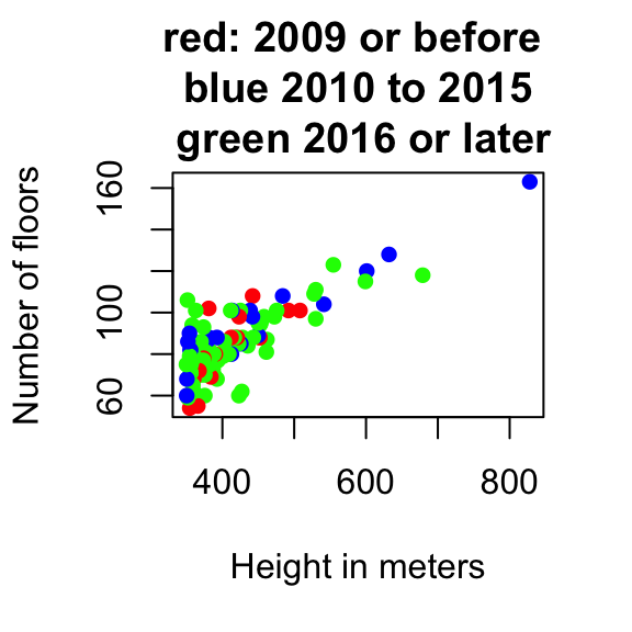
  • Generate a scatterplot. Can you think of a way to color it based on year, and reproduce this plot?
Show solution
  • Create an empty vector with the same length as the number of buildings
mycols <- rep(NA,nrow(df.building))
  • (Use R to tell which buildings were built in 2009 or before)
which(df.building$Year<=2009)
  • Set the corresponding element in the empty vector to the color red (recall, for subsetting, the which() function is not actually needed)
mycols[df.building$Year <= 2009] <- 'red'
  • Do the same for the other colors
mycols[(df.building$Year >= 2010)
  & (df.building$Year <= 2015)] <- 'blue'
mycols[df.building$Year >= 2016] <- 'green'

Alternatively, you can create three colors first and create index based on the year of the building, then use the index to subset the colors; this is beneficial since you can change the colors easily.

cols3 <- c('red', 'blue', 'green')
myindex <- ifelse(df.building$Year <= 2009, 1, NA)
myindex[(df.building$Year >= 2010)
  & (df.building$Year <= 2015)] <- 2
myindex[df.building$Year >= 2016] <- 3

# cols3 gives the same vector as mycols above
cols3[myindex]

NA values

  • NA is a special value that represents missing or unavailable entries when not in quotation marks
x <- c(3.5, 3.2, 3, NA)
length(x)
[1] 4
  • Most operations will return NA (e.g.: you don’t know the 4th value, so you cannot calculate the mean)
mean(x)
[1] NA
max(x)
[1] NA
sd(x)
[1] NA
  • To avoid the issue of getting NA’s when you perform calculations, you might want to exclude the NA values. some functions give you the option to remove NA; more generally, use na.omit()
mean(x,na.rm=T)
[1] 3.233333
max(x,na.rm=T)
[1] 3.5
mean(na.omit(x))
[1] 3.233333
  • To check for NA values, these syntax options don’t work as intended:
x
[1] 3.5 3.2 3.0  NA
x==NA  # NOT what we want!
[1] NA NA NA NA
which(x==NA)  # NOT what we want!
integer(0)
  • Instead, use is.na(x)
is.na(x)
[1] FALSE FALSE FALSE  TRUE
which(is.na(x))
[1] 4
  • NaN is also treated as NA; Inf is not treated as NA (represents infinity)

  • You should check the calculations and variable types when you see NA, NaN, or Inf

v1 <- c(1, 1, 0); v2 <- c(2, 0, 0); v1 / v2
[1] 0.5 Inf NaN
mean(v1/v2)
[1] NaN
is.na(v1/v2)
[1] FALSE FALSE  TRUE
as.numeric('4,000')
[1] NA

More on logicals

Composite logical statement: you can combine two or more logical statements together

  • ! NOT
  • & AND
  • | OR
x <- c(3.6, 2.8, 3.3, 1.2)
x>3
[1]  TRUE FALSE  TRUE FALSE
x>3 & x<3.5
[1] FALSE FALSE  TRUE FALSE
(x>3.5) | (x<2)
[1]  TRUE FALSE FALSE  TRUE
  • Recall, logical operators are the ones that return T/F
which(x < 3) # this is ok
which(x == 3)
which(x) # this is NOT ok
  • Operator %in% is another useful logical operator
subjects <- c('ENG', 'ENG', 'MAT', 'MAT', 'STAT', 'HIS')
subjects %in% c('MAT','STAT')
[1] FALSE FALSE  TRUE  TRUE  TRUE FALSE

Exercise: logical statements and subsetting

  1. Print the names and built years of the first 3 buildings
  2. Print the names of buildings in the United States
  3. Print the names of buildings in the United States AND also built after 2015
  4. Print the names of buildings in the United States OR in China
  5. Print the names and built years of buildings built between 2010 and 2015
  6. Print the names and built years of the buildings built in 2010 OR in 2015
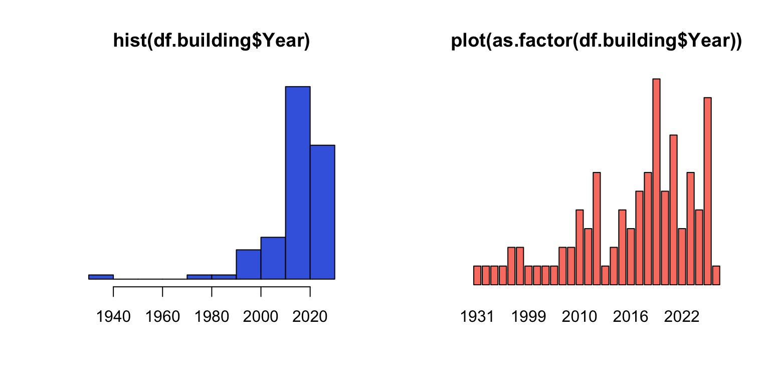
  7. Plot a histogram of the built year of the buildings. I’m interested to see there is a building built before 1940 - can you find out which building it is?
Show solution
# 1. First three buildings
df.building[1:3, c("Name", "Year")]

# 2. Buildings in the United States
df.building[df.building$Location == "United States", c("Name", "Year")]

# 3. Buildings in the United States built after 2015
df.building[df.building$Location == "United States" &
              df.building$Year > 2015, c("Name", "Year")]

# 4. Buildings in the United States or China
df.building[df.building$Location %in% c("United States", "China"),
            c("Name", "Year")]

# 5. Buildings built between 2010 and 2015, inclusive
df.building[df.building$Year >= 2010 & df.building$Year <= 2015,
            c("Name", "Year")]

# 6. Buildings built in 2010 or 2015
df.building[df.building$Year %in% c(2010, 2015), c("Name", "Year")]

# 7. Building built before 1940
df.building[df.building$Year < 1940, c("Name", "Year")]

par(mfrow=c(1,2))
hist((df.building$Year),
     col='royalblue',
     main='hist(df.building$Year)',
     xlab=NA,
     ylab=NA,
     yaxt='n')

plot(as.factor(df.building$Year),
     col='salmon',
     main='plot(as.factor(df.building$Year))',
     xlab=NA,
     ylab=NA,
     yaxt='n')

Comment: Bar graph is like histogram for discrete variables; recall, plot( ) gives a bar graph for factors