This part is based on the running dataset. It is a dataset that records my running mileage by day of the week. You’ll be using the pipe operator and data manipulation functions, so make sure you load relevant packages.
On average, which day of the week do I tend to run the most miles? Calculate the average mileage for Monday, Tuesday, etc. to compare.
        Week          Mon              Tue              Wed
 Length   :317   Min.   : 0.000   Min.   : 0.000   Min.   : 0.000
 N.unique :317   1st Qu.: 0.000   1st Qu.: 0.000   1st Qu.: 0.000
 N.blank  :  0   Median : 0.000   Median : 1.000   Median : 2.000
 Min.nchar:  6   Mean   : 1.508   Mean   : 1.915   Mean   : 2.256
 Max.nchar:  8   3rd Qu.: 2.000   3rd Qu.: 3.000   3rd Qu.: 4.000
                 Max.   :20.000   Max.   :14.000   Max.   :17.000
      Thu              Fri              Sat              Sun
 Min.   : 0.000   Min.   : 0.000   Min.   : 0.000   Min.   : 0.000
 1st Qu.: 0.000   1st Qu.: 0.000   1st Qu.: 0.000   1st Qu.: 0.000
 Median : 1.500   Median : 0.000   Median : 0.000   Median : 2.000
 Mean   : 2.164   Mean   : 2.071   Mean   : 1.909   Mean   : 4.078
 3rd Qu.: 4.000   3rd Qu.: 4.000   3rd Qu.: 2.500   3rd Qu.: 7.000
 Max.   :19.000   Max.   :12.000   Max.   :21.000   Max.   :26.200
Convert the data to the following long format and store it as a separate data frame (running.long). Note that your output might be sorted by Day (i.e., the first rows correspond to all the Monday data). Print out the first 5 rows of your data.
# A tibble: 7 × 2
  Day   average.miles
  <chr>         <dbl>
1 Sun            4.08
2 Wed            2.26
3 Thu            2.16
4 Fri            2.07
5 Tue            1.91
6 Sat            1.91
7 Mon            1.51
Print out the top 10 days when I ran the most miles (you should get the following information), using both running (wide format) and running.long (long format). Discuss which format is easier in this case.
Show solution
# wide format: difficult# maybe: manually sort through Monday to Sunday to find top 10running %>%arrange(desc(Mon)) %>%slice(1:10)
# long format: easyrunning.long %>%arrange(desc(Miles)) %>%slice(1:10)
# A tibble: 10 × 3
   Week     Day   Miles
   <chr>    <chr> <dbl>
 1 11/13/17 Sun    26.2
 2 1/14/19  Sun    26.2
 3 5/6/19   Sun    26.2
 4 1/6/20   Sun    26.2
 5 11/15/21 Sun    26.2
 6 4/8/19   Sat    21
 7 10/23/17 Sun    20
 8 11/26/18 Sun    20
 9 12/17/18 Mon    20
10 4/1/19   Sun    20
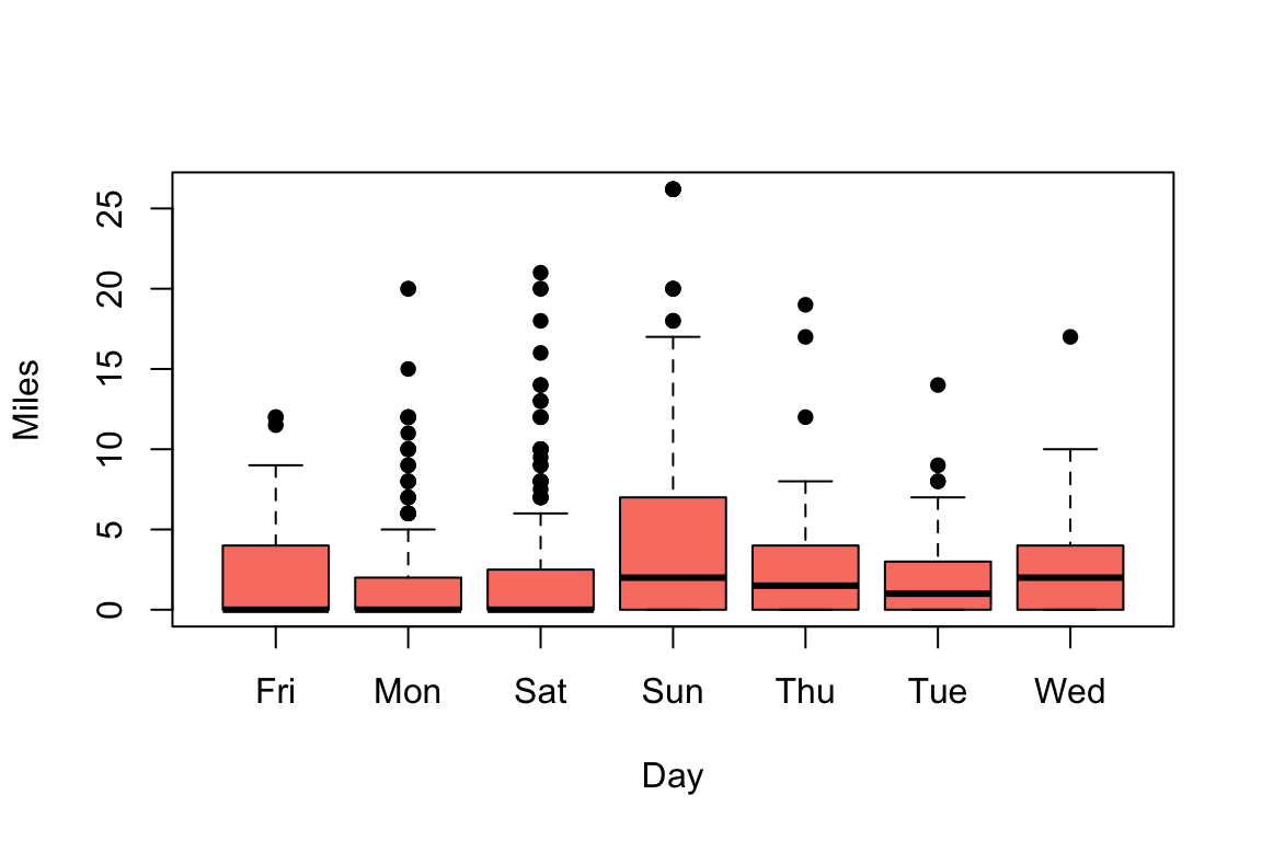
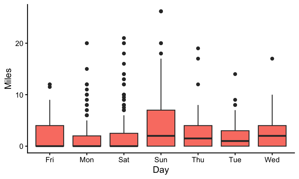
Reproduce the following two graphs with running.long (which is much easier than using the wide format!). They are essentially the same graph, but the first one is done with the base R boxplot function and the second one is done with ggplot2 (with theme_classic).
Take a look at the dataset USArrests in base R. Run the following code to extract the state names and store it as a separate variable in the data frame.
USArrests$state <-row.names(USArrests)
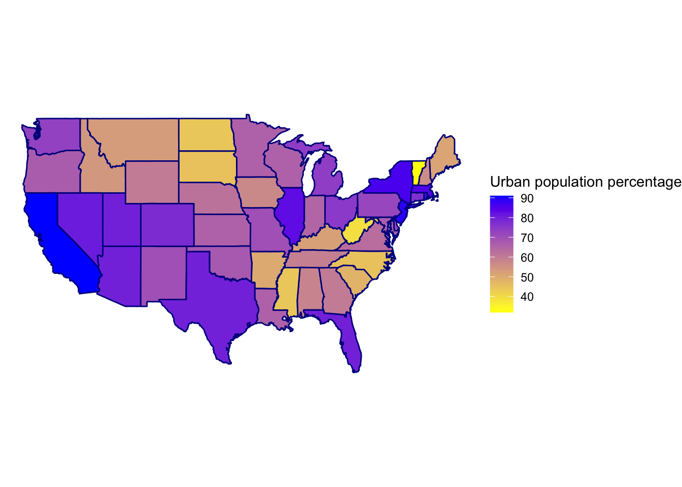
The following graph is generated using the maps package and based on the variable UrbanPop in the USArrests dataset. Reproduce this graph (you can visualize other variables in the USArrests dataset instead of UrbanPop, if you prefer). You can find sample code from Lecture 6 here.
Show solution
library(maps)USArrests$state <-row.names(USArrests) %>%tolower()mymap <-map_data(map="state")# Combine crime data to map datamymap <-left_join(mymap, USArrests, by=c('region'='state'))# Visualizemymap %>%ggplot(aes(x=long,y=lat,group=group, fill=UrbanPop)) +geom_polygon(color='darkblue') +coord_fixed(1.4) +theme_void() +labs(fill='Urban population percentage') +scale_fill_gradient(low="yellow", high="blue")