Show solution
stem(Cereal$Calories)
  The decimal point is 1 digit(s) to the right of the |

   8 | 074
  10 | 0178347777788
  12 | 090
  14 | 49
  16 | 00915
  18 | 225
20 | 4Homework 5
This part uses the Cereal dataset in the Lock5Data package. Make sure to load the relevant packages. The plots are shown below. For each one, write R code to reproduce it. Elements such as titles, labels, colors, and themes can differ, but make appropriate modifications instead of relying on defaults. The suggested ggplot theme is provided; you may use another theme. Open Show solution to see one possible solution.
Plot 1. (This is not a ggplot; the variable used is Calories)
stem(Cereal$Calories)
The decimal point is 1 digit(s) to the right of the |
8 | 074
10 | 0178347777788
12 | 090
14 | 49
16 | 00915
18 | 225
20 | 4Plot 2. (This is not a ggplot)
plot(Cereal$Calories,Cereal$Sugars,
     xlab='Calories per cup',
     ylab='Sugars (grams per cup)',
     pch=16)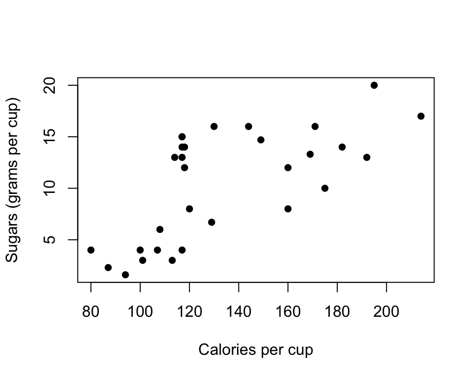
Plot 3. theme_classic()
Cereal %>%
  ggplot(aes(x=Calories,y=Sugars)) +
  geom_point() +
  theme_classic() +
  geom_vline(xintercept = 200,linetype='dashed')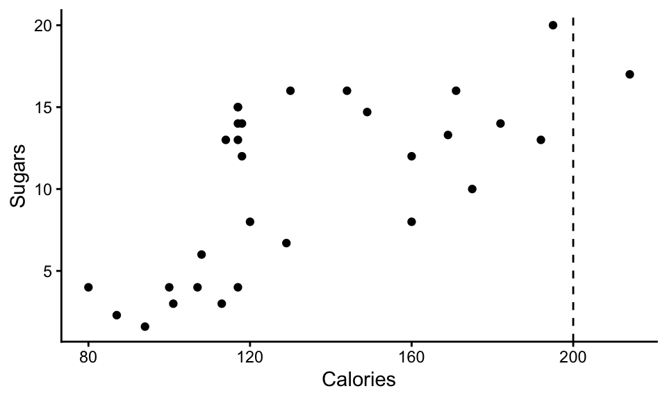
Plot 4. theme_bw()
Cereal %>%
  ggplot(aes(x=Calories,y=Sugars,color=Company)) +
  geom_point() +
  theme_bw() +
  labs(x='Calories per cup', y='Sugars (grams per cup)')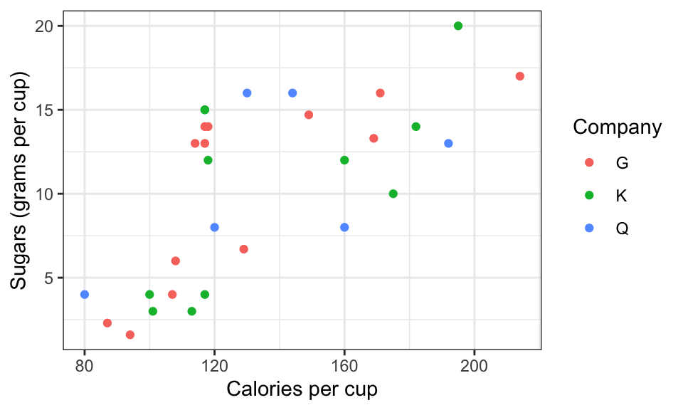
Plot 5. theme_bw()
Cereal %>%
  ggplot(aes(x=Calories,fill=Company)) +
        geom_histogram(binwidth=10,color='blue') +
        theme_bw()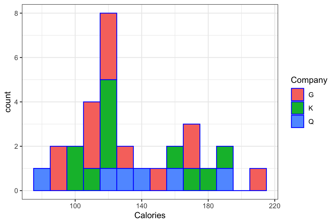
Plot 6. theme_minimal()
Cereal %>%
  ggplot(aes(x=Calories,y=Sugars,color=Fat)) +
  geom_point() +
  theme_minimal() +
  labs(x='Calories per cup', y='Sugars (grams per cup)') +
  scale_color_gradient(low="yellow",high="red")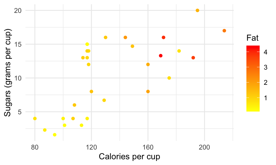
Plot 7. theme_minimal()
 Cereal %>%
  ggplot(aes(x=Calories,y=Sugars,label=Name)) +
  geom_label() +
  theme_minimal() +
  labs(x='Calories per cup', y='Sugars (grams per cup)')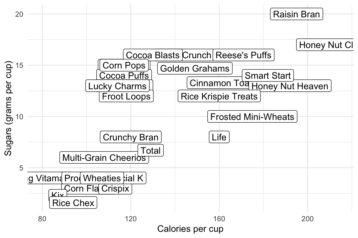
This part uses the UNICEF Changing Childhood Project data (the same dataset used in Lecture 5). It’s an open-ended exploration of the data, giving you practice handling a complicated dataset with tidyverse and generating visualizations with ggplot2. Think about what conclusions you can draw from the tables and visualizations, and write code to reproduce them. In addition, try other variables in the data to generate your own visualizations (see if you can find anything interesting!)
I used these variables:
COUNTRYNEW: countryAGE: age group: 1 = 15-19, 2 = 20-24, 3 = 40-44, 4 = 45-49, 5 = 50-54, 6 = 55-59, 7 = 60-64, 8 = 65-69, 9 = 70-74, 10 = 75-99.The table shows the top countries in terms of the percentage of respondents who trust the police “a lot.” The boxplot shows the univariate distribution of this percentage.
COUNTRYNEW: countryWP22096: trust in the country’s police to protect the respondent: 1 = a lot, 2 = a little, 3 = not at all, 8 = don’t know, 9 = refused.df.child %>%
filter(WP22096 %in% 1:3) %>%
group_by(COUNTRYNEW) %>%
summarise(percent1= mean(WP22096 == 1), .groups = "drop") %>%
arrange(desc(percent1)) # A tibble: 21 × 2
COUNTRYNEW percent1
<chr> <dbl>
1 Morocco 0.669
2 Zimbabwe 0.638
3 Germany 0.574
4 India 0.535
5 United States 0.530
6 Spain 0.519
7 United Kingdom 0.501
8 Indonesia 0.496
9 Mali 0.44
10 France 0.385
# ℹ 11 more rowsdf.child %>%
filter(WP22096 %in% 1:3) %>%
group_by(COUNTRYNEW) %>%
summarise(percent1= mean(WP22096 == 1), .groups = "drop") %>%
ggplot(aes(y = percent1)) +
geom_boxplot() +
theme_minimal() +
ggtitle("Percentage in a country who trust the police 'a lot'")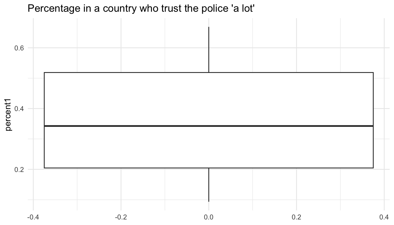
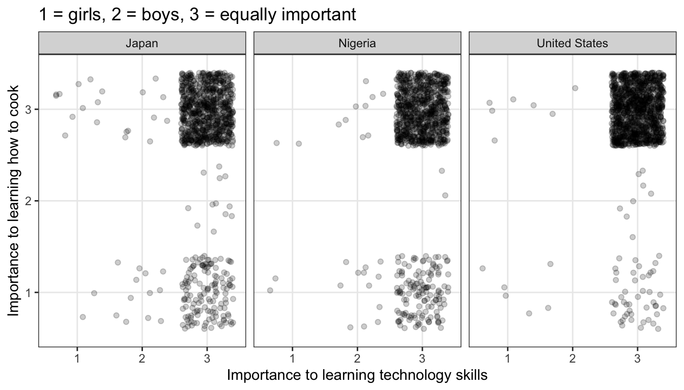
Compare responses from selective countries to the questions about technology skills (WP22078) and cooking (WP22079).
WP22078: whether it is more important for girls, boys, or equally important for both to learn how to use a smartphone, computer, or tabletWP22079: whether it is more important for girls, boys, or equally important for both to learn how to cook1 = girls, 2 = boys, 3 = equally important, 8 = don’t know, 9 = refused.df.child %>%
filter(COUNTRYNEW %in% c("United States", "Japan", "Nigeria")) %>%
filter(WP22078 %in% 1:3, WP22079 %in% 1:3) %>%
ggplot(aes(x = as.factor(WP22078), y = as.factor(WP22079))) +
geom_jitter(alpha = 0.2) +
facet_wrap(~COUNTRYNEW) +
theme_bw() +
labs(
title = "1 = girls, 2 = boys, 3 = equally important",
x = "Importance to learning technology skills",
y = "Importance to learning how to cook",
)
Create a new variable by adding up the following. They are all
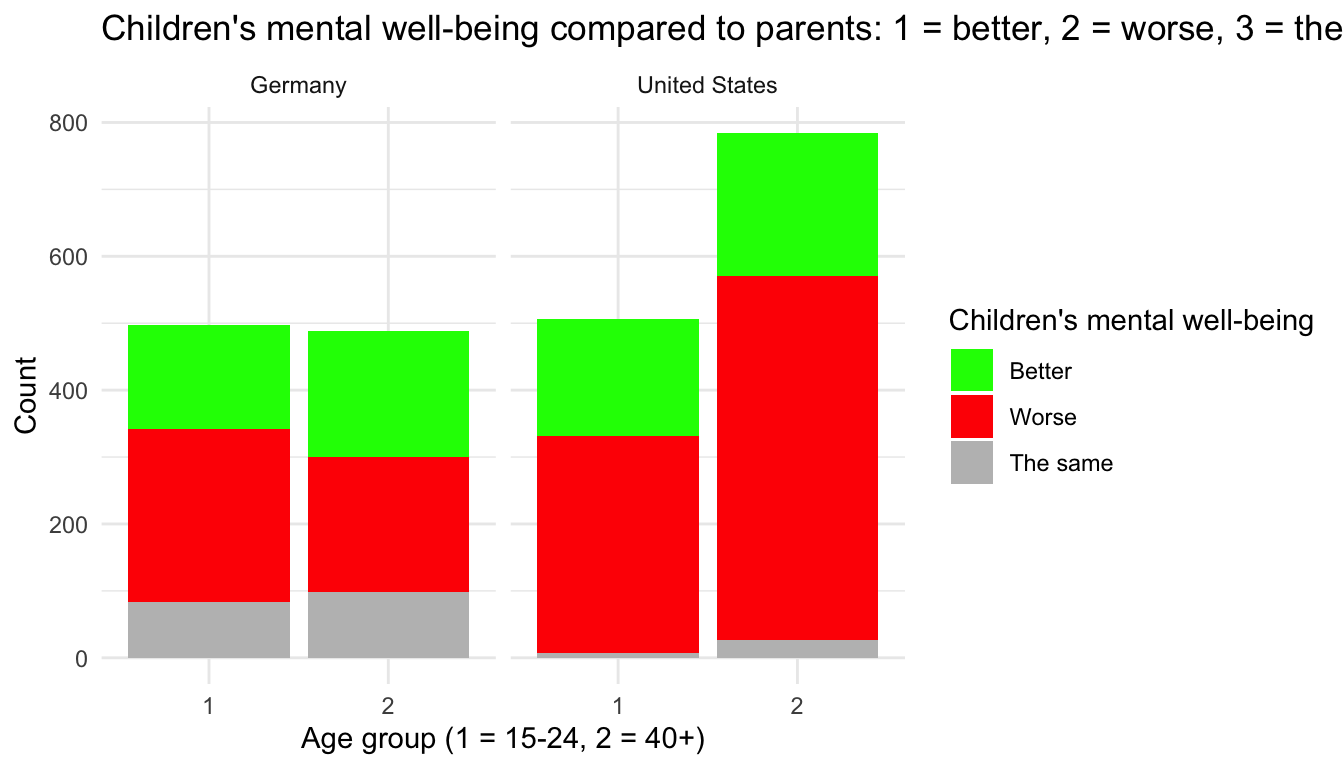
WP22140: Age; coded as ‘1’ = 15-24, ‘2’ = 40 or older.WP22118: whether children’s mental well-being is better or worse than in their parents’ time; coded as 1 = better, 2 = worse, 3 = the same, 8 = don’t know, 9 = refused.`df.child %>%
filter(WP22118 %in% 1:3, WP22140 %in% 1:2) %>%
filter(COUNTRYNEW %in% c("United States", "Germany")) %>%
ggplot(aes(x = as.factor(WP22140), fill = as.factor(WP22118))) +
geom_bar() +
scale_fill_manual(
values = c("1" = "Green", "2" = "Red", "3" = "Grey"),
labels = c("1" = "Better", "2" = "Worse", "3" = "The same")
) +
facet_wrap(~COUNTRYNEW) +
theme_minimal() +
labs(
x = "Age group (1 = 15-24, 2 = 40+)",
y = "Count",
fill = "Children's mental well-being"
) +
ggtitle("Children's mental well-being compared to parents: 1 = better, 2 = worse, 3 = the same")