Chapter 6
Exercise 6.1
In Exercise 5.6, we used the States data set to determine that there was a positive linear relationship between EDUCEXPE, the average educational expenditure per pupil, and TEACHPAY, the average salary of public school teachers in the state. In this exercise, create and interpret a model to predict EDUCEXPE from TEACHPAY.
- Verify that regression is appropriate in this case.
- Find the regression equation for predicting
EDUCEXPEfromTEACHPAY. - Interpret the value of the slope in context, using language that someone who has not taken statistics would understand.
- Interpret the value of the intercept in context, or indicate why it is not meaningful.
- What is the predicted educational expenditure for a state with teacher pay of $40,000?
- Is it appropriate to use the regression equation to predict educational expenditure for a state with teacher pay of $80,000?
- Report the value of \(R\) and interpret it in context.
Show solution
EDUCEXPEandTEACHPAYare scale/ratio variables, and the scatterplot indicates that the pattern is effectively approximated by a line.- \(\widehat{EDUCEXPE} = 0.276(TEACHPAY) - 3372.988\).
- A one-dollar increase in average teacher salary corresponds to an average increase of about 28 cents in per-pupil educational expenditure.
- The intercept is not meaningful because no state’s average teacher salary is close to $0.
- \(0.276(40{,}000) - 3372.988 = \$7{,}667.01\).
- No. \(80{,}000\) is well beyond the largest teacher salary value in the data used to create the model.
- \(R = .72\), indicating a strong correlation between actual and predicted educational expenditures.
Exercise 6.3
Using the NELS data set, investigate whether twelfth-grade math achievement (ACHMAT12) can be predicted from eighth-grade socioeconomic status (SES). Create a scatterplot of ACHMAT12 by SES with the regression line and use the results to answer the following.
- Determine whether regression is appropriate for predicting
ACHMAT12fromSES. - What is the regression equation?
- Is there a meaningful interpretation of the slope? If so, explain what additional information it provides.
- Is there a meaningful interpretation of the y-intercept? If so, explain what additional information it provides.
- What is the predicted twelfth-grade math achievement score for a student with
SES = 20? - For the first student in the NELS data set (
ID = 1), what is the actual twelfth-grade math achievement score? - For this student, what is the predicted twelfth-grade math achievement score?
Show solution
- Both variables are interval-level, and the scatterplot pattern is sufficiently modeled by a line.
- \(\widehat{ACHMAT12} = 0.368(SES) + 50.123\).
- Each one-point increase in SES is associated with an average increase of 0.368 points in twelfth-grade math achievement.
- A student with
SES = 0is predicted to score 50.123 in twelfth-grade math achievement. - The predicted score is 57.483.
- The actual score is 59.69.
- The predicted score is 58.59.
Exercise 6.4
Use the Impeach data set to perform a simple linear regression analysis predicting a senator’s conservatism (CONSERVA) from the state voter support for Clinton (SUPPORTC).
- Create a scatterplot and verify that the data have an approximately linear shape.
- What is the correlation, \(r\), between conservatism and state voter support for Clinton?
- What is the value of \(R\), a measure of the goodness of fit? Describe the goodness of fit.
- Write the regression equation for predicting conservatism (\(Y\)) from state voter support for Clinton (\(X\)).
- Interpret the slope in context.
- Interpret the y-intercept, or explain why it is not meaningful.
- Use the regression equation to predict conservatism for a senator whose state gave Clinton 50 percent of the vote in the 1996 presidential election.
Show solution
- The shape is not exactly linear, but no other simple curve provides a better approximation.
- \(r = -.447\).
- \(R = .447\), indicating a moderate-to-strong goodness of fit.
- \(\widehat{CONSERVA} = -2.488(SUPPORTC) + 164.911\).
- Each one-percentage-point increase in state voter support for Clinton is associated with an average 2.488-point decrease in the senator’s conservatism rating.
- The intercept is not meaningful because the data include no states with voter support near zero; the lowest support value was above 30%.
- \(-2.488(50) + 164.911 = 40.51\).
Exercise 6.5
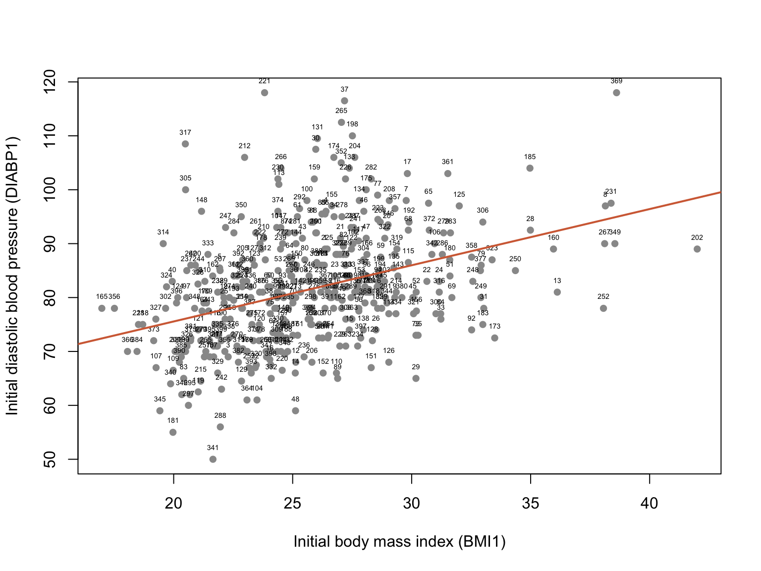
The following scatterplot, created using variables from the Framingham data set, shows the relationship between initial body mass index (BMI1) and initial diastolic blood pressure (DIABP1). Points are labeled by the person’s ID number. Use the scatterplot to answer the following questions.
- Is linear regression appropriate for analyzing the relationship? Explain.
- Is the slope positive, negative, or near zero? What does that tell you about the relationship?
- Use the regression line to estimate initial diastolic blood pressure for a person with an initial BMI of 19.
- Explain why the regression model should not be used to estimate initial diastolic blood pressure for a person with an initial BMI of 50.
Show solution
- Yes. Both variables are ratio-level, and the data are effectively modeled by a line, although a few outliers warrant investigation.
- The slope is positive: adults with relatively high BMI tend also to have relatively high diastolic blood pressure.
- Approximately 75 mmHg.
- A BMI of 50 is above the highest value measured in the data set, so using the model there would be extrapolation.
Exercise 6.8
In Exercise 6.1, a model was created to predict EDUCEXPE from TEACHPAY. Use that model to examine the residuals for Alabama, the first state in the data set.
- What is the predicted average educational expenditure for Alabama?
- What is Alabama’s actual average educational expenditure?
- What is the value of the residual?
- Does the model overpredict or underpredict
EDUCEXPEfor Alabama?
Show solution
- \(7{,}125.70\).
- \(6{,}300\).
- The residual is \(-825.70\).
- The model overpredicts Alabama’s educational expenditure.
Exercise 6.13
In this exercise, use the NELS data set to create a model predicting socioeconomic status (SES) from eighth-grade computer ownership (COMPUTER), a dichotomous variable.
- What is the regression equation for predicting SES from computer ownership?
- Interpret the slope in context.
- Interpret the intercept in context, or explain why it is not meaningful.
- Use the equation to predict SES for those who owned a computer in eighth grade.
- Use the equation to predict SES for those who did not own a computer in eighth grade.
- Use Jamovi to find the mean SES of those who did and did not own a computer in eighth grade.
- Is it ever not meaningful to interpret the intercept when the independent variable is dichotomous?
Show solution
- \(\widehat{SES} = 4.83(COMPUTER) + 16.144\).
- Students who owned a computer in eighth grade have an average SES 4.83 points higher than those who did not.
- The intercept, 16.14, is the predicted mean SES for students who did not own a computer in eighth grade (
COMPUTER = 0). - For owners, the predicted SES is \(4.83(1) + 16.144 = 20.97\).
- For non-owners, the predicted SES is \(4.83(0) + 16.144 = 16.14\).
- Comparing means gives those same group means: 20.97 for computer owners and 16.14 for non-owners.
- Yes. The intercept is meaningful when one category is coded 0. If neither category is coded 0, the intercept does not represent either group’s mean.
Exercise 6.14
Students in an introductory college statistics course took the SATS (Survey of Attitudes Toward Statistics). A regression model predicted VALUE (attitudes about the usefulness, relevance, and worth of statistics in personal and professional life, rated as the average of several 1-to-7 Likert-scale items) from GENDER, coded 1 = male and 2 = female. The regression equation is \(\widehat{VALUE} = .573(GENDER) + 4.059\). Use the equation and coding to answer the questions.
- What is the sign of the correlation between
GENDERandVALUE? - Which gender tended to give a higher rating to the value of the course?
- What is the predicted
VALUEscore for females? - What is the average
VALUEscore for males?
Show solution
- Positive, as indicated by the positive slope.
- Females.
- \(.573(2) + 4.059 = 5.21\).
- \(.573(1) + 4.059 = 4.63\).
Exercise 6.16
If there is a positive linear correlation between \(X\) and \(Y\), then the regression equation for predicting \(Y\) from \(X\) will have a:
- Positive slope
- Negative slope
- Positive y-intercept
- Negative y-intercept
Show solution
- Positive slope.
Exercise 6.20
During the semester, students in a statistics class provided their average weekly study time and course grade (on a 0.0-to-4.0 scale). The regression equation for predicting grade from hours studied was \(\widehat{Y} = 1.2X + 0.3\). If a student studies 3 hours per week on average, what is her predicted numerical course grade?
- 2.25
- 3.90
- 3.60
- Cannot be determined from the data
Show solution
- \(1.2(3) + 0.3 = 3.90\).
Exercise 6.21
Given the scenario in Exercise 6.20, which conclusion is warranted?
- For each additional hour of study per week, the predicted grade increases by 1.2 on average.
- For each additional hour of study per week, the predicted grade increases by 0.3 on average.
- For each additional hour of study per week, the predicted grade decreases by 1.2 on average.
- For each additional hour of study per week, the predicted grade decreases by 0.3 on average.
Show solution
- For each additional hour of study per week, the predicted grade increases by 1.2 points on average. The 1.2 is the regression slope.
Exercise 6.22
The correlation between exhaustion level and performance on an essay exam was \(r = -.90\). If Alejandro scores below the mean on exhaustion level, it is likely that he will score:
- Above the mean on the essay exam
- Below the mean on the essay exam
- On the mean on the essay exam
- In an unpredictable way on the essay exam
Show solution
- Above the mean on the essay exam. With a strong negative correlation, a below-average exhaustion score tends to be paired with an above-average exam performance score.
Exercise 6.24
The scatterplot below shows the relationship between \(X\) and \(Y\) for two groups. Group 1 is shown with triangles, and Group 2 is shown with circles.
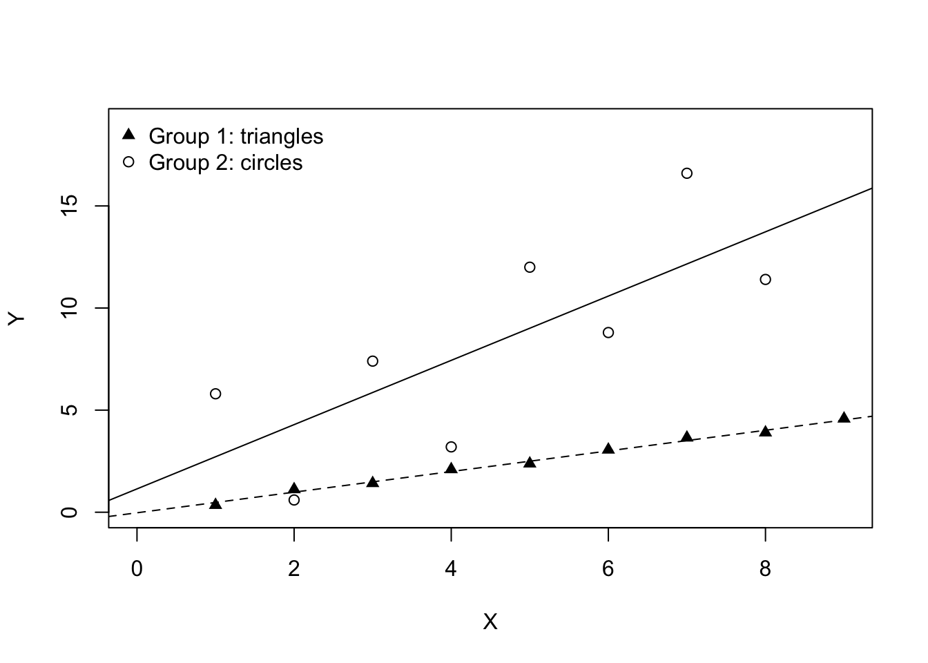
- Match each group with the most plausible value for its Pearson’s correlation coefficient: 1.25, 0.96, 0.87, -0.87, -0.96, -1.25
- Match each group with the most plausible value for its slope of the regression line: 1.9, 0.49, 0, -0.49, -1.9
Show solution
Group 1 has the stronger positive linear relationship because its points lie more closely around its fitted line (0.96), while Group 2’s correlation is weaker because its points are more scattered (0.87).
Group 2 has the steeper slope (1.9); Group 1 (triangles) has a smaller slope (0.49).