R code (optional)
# A tibble: 5 Ă— 3
Pos Counts Frequency
<chr> <int> <dbl>
1 C 36 0.152
2 PF 52 0.219
3 PG 43 0.181
4 SF 53 0.224
5 SG 53 0.224
STAT117: Introduction to Statistics
A simple, intuitive example: consider rolling a fair, six-sided die 🎲
What is the probability that you roll a 2?
What is the probability that you do not roll a 2?
What is the probability that you roll a number smaller than or equal to 4?
The answers should be very intuitive, but think about how you arrived at the answers precisely.
When we perform a random experiment (ex: roll a die), we can have different outcomes (ex: 1, 2, 3, 4, 5, 6).
Example: the event “rolling a number less than or equal to 4” is the collection of outcomes {1, 2, 3, 4}.
Example: the complement of the event “rolling a number less than or equal to 4” is the event “rolling a number greater than 4”, which is the collection {5, 6}.
For example, the events “rolling a 1” and “rolling a 2” are disjoint because they cannot occur at the same time.
Example: P(rolling < 5) = 4/6 comes from the fact that there are 4 outcomes in the event {1, 2, 3, 4} and 6 total outcomes.
Example: P (not rolling 2) = 1 – P ( rolling 2) = 1 – 1/6
Example: P (rolling 1 or rolling > 4) = P (rolling 1) + P (rolling > 4) = 1/6 + 2/6
Pos) in the NBAPlayers2024 dataset (download). Position codes are C (center), PF (power forward), PG (point guard), SF (small forward), and SG (shooting guard).# A tibble: 5 Ă— 3
Pos Counts Frequency
<chr> <int> <dbl>
1 C 36 0.152
2 PF 52 0.219
3 PG 43 0.181
4 SF 53 0.224
5 SG 53 0.224
Assume that one player is selected at random from the dataset. Find the probability that the player is:
C) and point guards (PG) in the NBAPlayers2024 dataset. Player ages are grouped into three categories.nba_position_age <- NBAPlayers2024 %>%
filter(Pos %in% c("C", "PG")) %>%
mutate(
AgeGroup = cut(
Age,
breaks = c(18, 24, 29, Inf),
labels = c("19-24", "25-29", "30+")
)
) %>%
count(Pos, AgeGroup, name = "Count")
ggplot(nba_position_age, aes(x = Pos, y = Count, fill = AgeGroup)) +
geom_col(position = "dodge") +
geom_text(
aes(label = Count),
position = position_dodge(width = 0.9),
vjust = -0.3
) +
labs(
x = "Player position",
y = "Count",
fill = "Age group"
) +
theme_minimal()
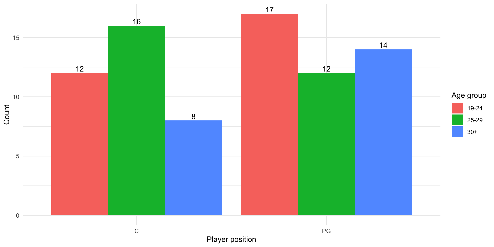
If I randomly select a Center, what is the chance that he is 30+ years old? What if I randomly select a Point Guard?
Random sample means that each person in the population has an equal chance of being selected. A true random sample is often difficult to obtain and we should always be critical about sampling bias.
From a recent article about voting polls: Why haven’t polls overstated Democrats’ chances in recent midterms? One factor seems to be that President Trump excels among a relatively disengaged group of voters who are unlikely to respond to surveys — but who are also unlikely to vote in midterm elections. As a result, the polls — and Democrats — do better in lower-turnout elections, when a highly engaged, poll-taking, Democratic-leaning set of voters shows up. By contrast, in the last three presidential elections, many of these hard-to-reach Trump supporters did show up to vote, creating problems for pollsters.
Sometimes the randomness comes from the experiment itself (e.g., rolling a die, attempting a free throw). The randomness can also come from the sampling process, as the point of a random sample is that you don’t know who might end up in the sample.
Example: if 38 percent of households (in a certain region) own a cat, you might say that the probability of owning a cat is 0.38. What is meant that you imagine selecting a household at random; there is a 38% chance that the household you happen to select owns a cat.
Example: the probability of rolling a 2 on a fair die is 1/6 (or 0.167). You could also understand this as: if you roll a large number of fair dice, about 16.7 percent of them will be a 2.
Example: a statement like “the vaccine is 98% effective” can be interpreted as: when administered to a large number of people, the vaccine is effctive for 98 percent of them.