Chapter 6: Simple Linear Regression

STAT117: Introduction to Statistics

Introduction

You want to predict something (e.g., predict stock prices; predict a person’s marathon finish time; predict a student’s social economic status SES)

In reality, the main goal can be the prediction itself, or can be understanding what variables are important for making the prediction.

  1. The “something” you are predicting:

  2. The variable(s) you would use to make a prediction:

  • For instance, what variables would you use to predict a student’s SES?


Introduction

We’ll only cover these two cases:

  • Case 1: Y is numeric and X is scale (Covariate)
  • Case 2: Y is numeric and X is dichotomous (Factor)

Jamovi procedure: Analyze – Regression – Linear Regression; Whatever you are predicting goes in the Dependent box. Numeric predictors go in the Covariates box; categorical predictors go in the Factors box.

Exercise

Identify the dependent (Y) variable. For the independent (X) variable, label it as covariate or factor.

  1. Use a student’s SAT score to predict the student’s GPA in college


  1. Predict a student’s satisfaction with Drew’s dining service by whether the student is an international student


  1. Predict your future salary based on your GPA in college


  1. Use achmat08 to predict achrdg08


Show solution
  1. Dependent (Y): College GPA. Independent (X): SAT score, a covariate.
  2. Dependent (Y): Satisfaction with Drew’s dining service. Independent (X): International-student status, a factor.
  3. Dependent (Y): Future salary. Independent (X): College GPA, a covariate.
  4. Dependent (Y): achrdg08. Independent (X): achmat08, a covariate.

Case 1: Numeric predictor

SES and achmat08

R code (optional)
nels <- haven::read_sav("../../../../dataset/NELS.sav")

plot(
  nels$achmat08,
  nels$ses,
  xlab = "Math achievement in 8th grade (achmat08)",
  ylab = "SES",
  pch = 16
)

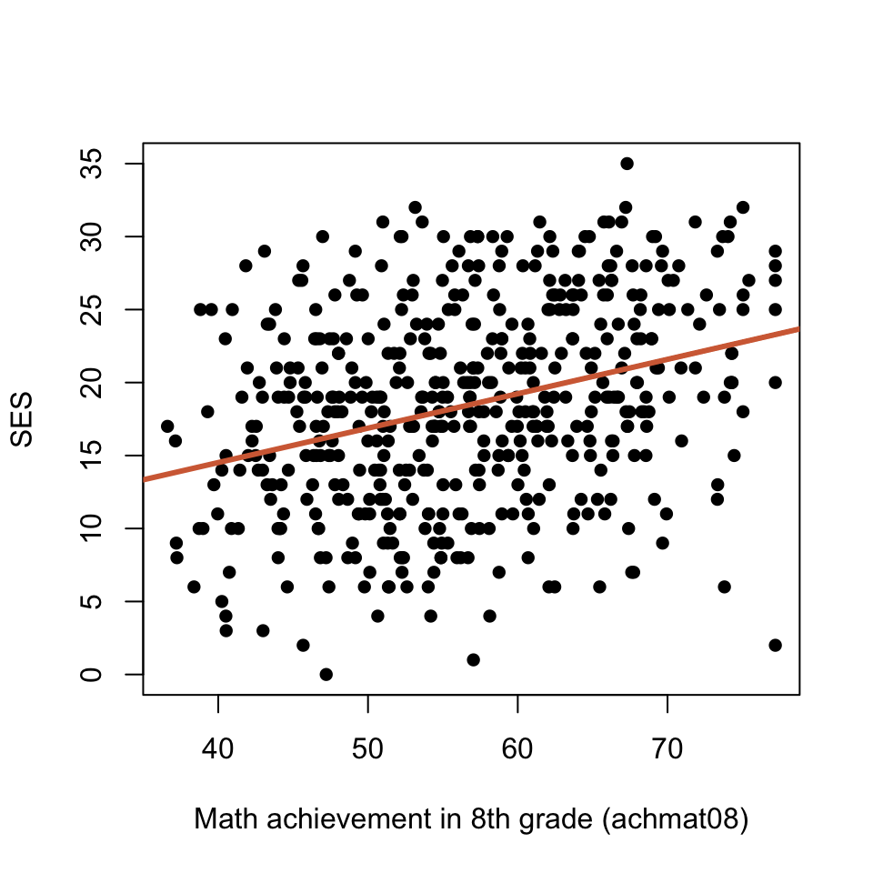
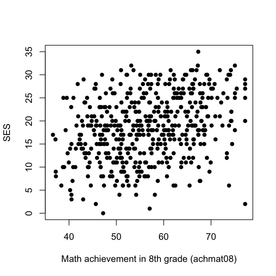
Scatterplot of eighth-grade math achievement and socioeconomic status, with a fitted regression line

  • Review: is there a relationship between achmat08 and SES? (Pearson r = 0.318)

  • Can you provide an estimate of SES, if a student’s achmat08 score is

    • around 45?
    • around 70?

Regression line

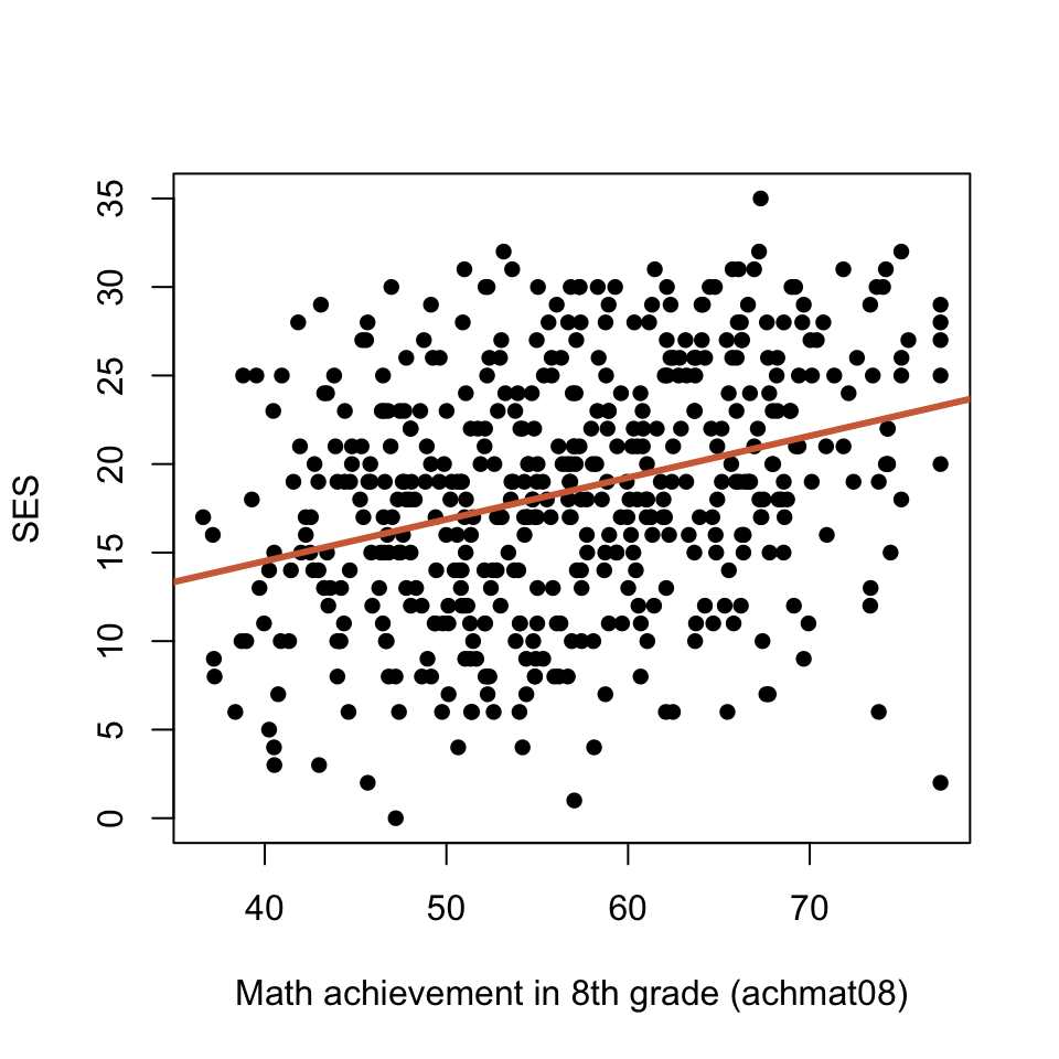
The goal is to find the line that “best fits” the data. The (least squares) regression line minimizes the total “distance” of each point to the line (where distance is measured by the squared difference).
R code (optional)
nels <- haven::read_sav("../../../../dataset/NELS.sav")

plot(
  nels$achmat08,
  nels$ses,
  xlab = "Math achievement in 8th grade (achmat08)",
  ylab = "SES",
  pch = 16
)

abline(lm(ses ~ achmat08, data = nels), col = "#D36B43", lwd = 3)

Scatterplot of eighth-grade math achievement and socioeconomic status, with a fitted regression line

Regression line

Model Fit Measures

Model R R\(^2\)
1 0.318 0.101

Model Coefficients - ses

Predictor Estimate SE t p
Intercept 5.082 1.8064 2.81 .005
achmat08 0.236 0.0315 7.49 <.001
  • Recall, the form of a line is given by:

  • Important: HAT notation is used to denote predicted values. 🧢

Predictions

\(\hat{Y} = 5.082 + 0.236 \cdot X\)

\(\hat{SES} = 5.082 + 0.236 \cdot achmat08\)

  • What is the predicted SES for a student with an achmat08 score of 45?


Be cautious about predicting out of the range of X!

  • What is the predicted SES for a student with an achmat08 score of 10?
Show solution
  • For achmat08 = 45, \(\widehat{SES} = 5.082 + 0.236(45) = 15.702\), or about 15.70.
  • For achmat08 = 10, the equation gives \(\widehat{SES} = 5.082 + 0.236(10) = 7.442\), or about 7.44. However, 10 is outside the observed range of achmat08, so this is an extrapolation and may not be reliable.

Residuals

\(\hat{SES} = 5.082 + 0.236 \cdot achmat08\)

Selected students from the NELS dataset:

Student ID achmat08 ses
374 44.80 21
489 44.80 20
67 70.04 27
  • Residual = actual - predicted = ses - \(\hat{SES}\)

  • What is the residual for student with ID 374?


  • Exercise: calculate the residuals for students with IDs 489 and 67.
Show solution

Residual = actual SES \(-\) predicted SES.

  • ID 374: \(21 - [5.082 + 0.236(44.80)] = 5.345\), or about 5.35. The model underpredicts SES.
  • ID 489: \(20 - [5.082 + 0.236(44.80)] = 4.345\), or about 4.35. The model underpredicts SES.
  • ID 67: \(27 - [5.082 + 0.236(70.04)] = 5.389\), or about 5.39. The model underpredicts SES.

Interpretations

Model Coefficients - ses

Predictor Estimate SE t p
Intercept 5.082 1.8064 2.81 .005
achmat08 0.236 0.0315 7.49 <.001

\(\hat{SES} = 5.082 + 0.236 \cdot achmat08\)

  • Slope


  • Intercept


Show solution
  • Slope (0.236): For each one-point increase in eighth-grade math achievement, predicted SES increases by 0.236 points, on average.
  • Intercept (5.082): “A student with an eighth-grade math achievement score of 0 is predicted to have an SES score of 5.082.” This is not interpretable because a score of 0 is outside the observed range of achmat08.

Regression and scatterplot

R code (optional)
nels <- haven::read_sav("../../../../dataset/NELS.sav")

plot(
  nels$achmat08,
  nels$ses,
  xlab = "Math achievement in 8th grade (achmat08)",
  ylab = "SES",
  pch = 16
)

abline(lm(ses ~ achmat08, data = nels), col = "#D36B43", lwd = 3)

Scatterplot of eighth-grade math achievement and socioeconomic status, with a fitted regression line

Example: Icecream

(Icecream.sav) We want to use temperature to predict the number of ice cream bars sold.

  1. Write down the regression line.

  2. Provide the value of the intercept and give an interpretation.

  3. Provide the value of the slope and give an interpretation.

  4. For a day with a temperature of ____ Fahrenheit, how many ice cream bars do you estimate to be sold?

  5. For day ID=12, are we over-predicting or under-predicting? Calculate the residual.

Show solution
  1. The regression equation is \(\widehat{BARSOLD} = 75.779 + 1.1804(TEMP)\).
  2. The intercept is 75.779: when temperature is 0°F, the model predicts about 76 bars sold. This is not interpretable because a temperature of 0°F is outside the observed range of temperatures.
  3. The slope is 1.1804: for each 1°F increase in temperature, predicted ice cream bar sales increase by about 1.18 bars, on average.
  4. For example, at 56°F the predicted sales are \(75.779 + 1.1804(56) = 141.88\), or about 142 bars. Be cautious since a temperature of 56°F is out of the range of the data.
  5. For ID 12, temperature is 75°F and actual sales are 167 bars. The predicted sales are \(75.779 + 1.1804(75) = 164.31\), so the residual is \(167 - 164.31 = 2.69\) bars. The model underpredicts sales for this day.

Case 2: dichotomous predictor

SES and nursery school (0=no, 1=yes)

R code (optional)
nels <- haven::read_sav("../../../../dataset/NELS.sav")

plot(
  nels$nursery,
  nels$ses,
  xlab = "Nursery school attendance (nursery)",
  ylab = "SES",
  pch = 16
)

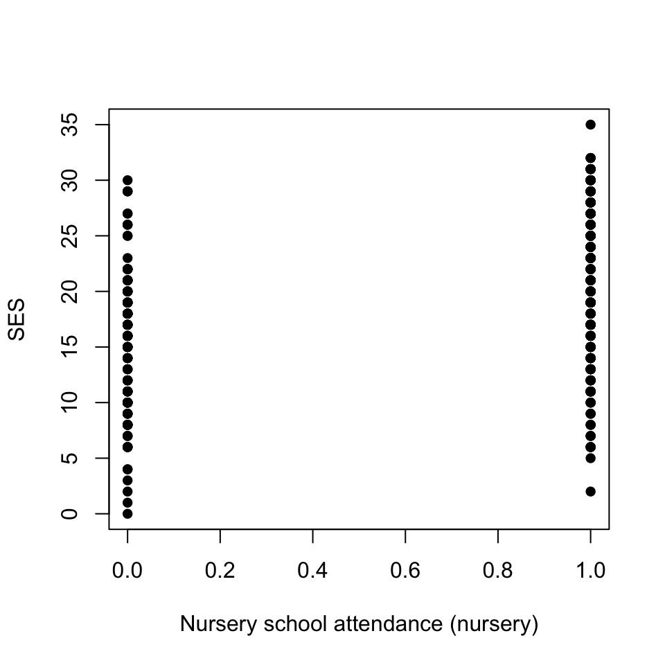
Scatterplot of nursery school attendance and socioeconomic status, with a fitted regression line

Can you estimate a student’s SES if the student…
  • has not attend nursery school?
  • has attended nursery school?

General idea

Predict SES based on Nursery: essentially, this means we predict SES for the two values of Nursery:

  • If Nursery = Yes, we predict SES to be ________
  • If Nursery = No, we predict SES to be ________
Show descriptives

(Analyses -> Exploration -> Descriptives)

Descriptives

Statistic nursery ses
N No 139
Yes 281
Mean No 15.1
Yes 20.7
Median No 16.0
Yes 21.0

We can get the same results from a regression analysis!

Example: Nursery

Use regression to predict SES using Nursery (coded as 0=No, 1=Yes).

Make sure to put Nursery as a factor! (For dichotomous predictors, you can get the same correct coefficients if you put it as a covariate, but this is not recommended, as you will get incorrect information when the variable is nominal or ordinal, or is coded in a non-standard way.)

  1. Write down the regression line.

  2. For a student who did attend nursery, what is the estimated SES?

  3. For a student who did not attend nursery, what is the estimated SES?

  4. Provide the value of the intercept and give an interpretation.

  5. Provide the value of the slope and give an interpretation.

  6. For student with ID=1, what is the residual? Are we over-predicting or under-predicting?


Show solution

The model uses 420 students with non-missing SES and Nursery values. Because Nursery is a factor, the intercept is the mean SES for students who did not attend nursery, and the slope is the difference between the Yes and No group means.

  • a) Regression line: \(\widehat{SES} = 15.072 + 5.665(NurseryYes)\), where NurseryYes is 0 for No and 1 for Yes.
  • b) Attended nursery: \(15.072 + 5.665(1) = 20.737\). The estimated SES is about 20.74.
  • c) Did not attend nursery: \(15.072 + 5.665(0) = 15.072\). The estimated SES is about 15.07.
  • d) Intercept: 15.072 is the predicted mean SES for students who did not attend nursery school.
  • e) Slope: 5.665 is the difference in predicted mean SES between students who attended nursery and those who did not. Students who attended nursery have a predicted SES about 5.66 points higher, on average.
  • f) Student ID 1: This student attended nursery and has actual SES 23. The prediction is 20.737, so the residual is \(23 - 20.737 = 2.263\). The positive residual means the model underpredicts this student’s SES.

Example: Computer

Use regression to predict SES by whether or not the family owned a computer (coded as 0=No, 1=Yes).

  1. Write down the regression line.

  2. For a student whose family had a computer, what is the estimated SES?

  3. For a student whose family did not have a computer, what is the estimated SES?

  4. Provide the value of the intercept and give an interpretation.

  5. Provide the value of the slope and give an interpretation.

  6. For student with ID=1, what is the residual? Are we over-predicting or under-predicting?


Show solution

The model uses 500 students with non-missing SES and computer values. Because computer is a factor, the intercept is the mean SES for students whose families did not own a computer, and the slope is the difference between the Yes and No group means.

  • a) Regression line: \(\widehat{SES} = 16.144 + 4.830(ComputerYes)\), where ComputerYes is 0 for No and 1 for Yes.
  • b) Family had a computer: \(16.144 + 4.830(1) = 20.975\). The estimated SES is about 20.97.
  • c) Family did not have a computer: \(16.144 + 4.830(0) = 16.144\). The estimated SES is about 16.14.
  • d) Intercept: 16.144 is the predicted mean SES for students whose families did not own a computer.
  • e) Slope: 4.830 is the difference in predicted mean SES between students whose families owned a computer and those whose families did not. Students whose families owned a computer have a predicted SES about 4.83 points higher, on average.
  • f) Student ID 1: This student’s family had a computer and actual SES is 23. The prediction is 20.975, so the residual is \(23 - 20.975 = 2.025\). The positive residual means the model underpredicts this student’s SES.

Example: slope interpretation

The following table is adapted from a 2020 publication, Training for a (half‐)marathon: Training volume and longest endurance run related to performance and running injuries.

For each predictor, interpret the number given in the “Estimate” column.

Significant predictors of marathon finish time (in min):

Predictor Estimate
Sex (female) 10.78
BMI (kg/m²) 1.58
Running experience (years) -0.42
Longest endurance run (km): <25 13.44