Chapter 5: Bivariate Relationships

STAT117: Introduction to Statistics

Introduction

Among runners (StatChat discussion), is there a relationship between finishing time and gender? Between finishing time and BMI? Between age categories and runner types (e.g., elite, intermediate, recreational)?

In this chapter, we look at TWO variables. We want to ask: do they have an association? For different groups of people (e.g., by gender or by age bracket), does the distribution of one variable (e.g., finishing time) differ? If there is an association, how strong is it?

How you answer these questions vary largely based on the measurement type of the variables. You should use appropriate statistics (e.g., correlation coefficients and percentages comparisons) and visualizations (e.g., scatterplots).

⚠️ Correlation does not imply causation.

Bivariate relationship WITHOUT nominal variables

Scatterplot 📊

A scatterplot is a bivariate graph of two numeric variables.

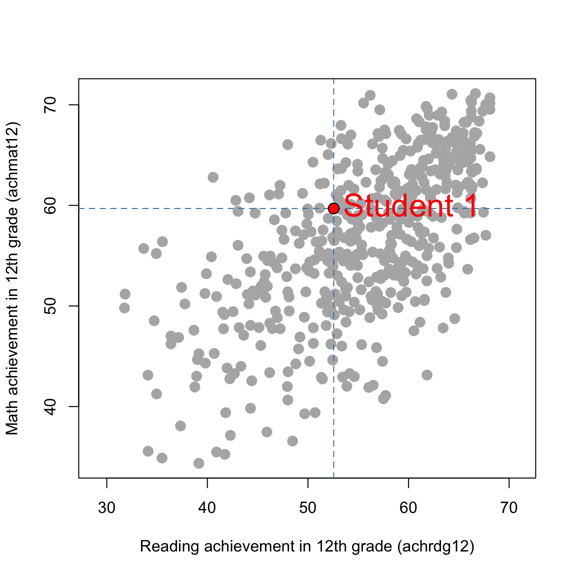
Example: In the NELS dataset, (achrdg12, achmat12) values can be considered in pairs:

  • Student 1: (52.56, 59.69)
  • Student 2: (53.12, 55.36)
  • Student 3: (54.79, 56.73)
  • \(\ldots\)

The scatterplot (next page) shows 500 dots, each corresponding to one student in the dataset. The highlighted dot represents Student 1.

NELS achievement scatterplot

R code (optional)
nels <- haven::read_sav("../../../../dataset/NELS.sav")

plot(
  nels$achrdg12,
  nels$achmat12,
  xlab = "Reading achievement in 12th grade (achrdg12)",
  ylab = "Math achievement in 12th grade (achmat12)",
  pch = 16,
  col = "gray70",
  asp = 1,
  cex = 1.5
)

abline(v = 52.56, lty = 2, col = "steelblue")
abline(h = 59.69, lty = 2, col = "steelblue")
points(52.56, 59.69, pch = 21, cex = 1.5, bg = "red", col = "black")
text(52.56, 59.69, labels = "Student 1", pos = 4, col = "red", cex=2)

Other Scatterplot Examples

Here are more examples of scatterplots (see StatChat2)

Linear relationship

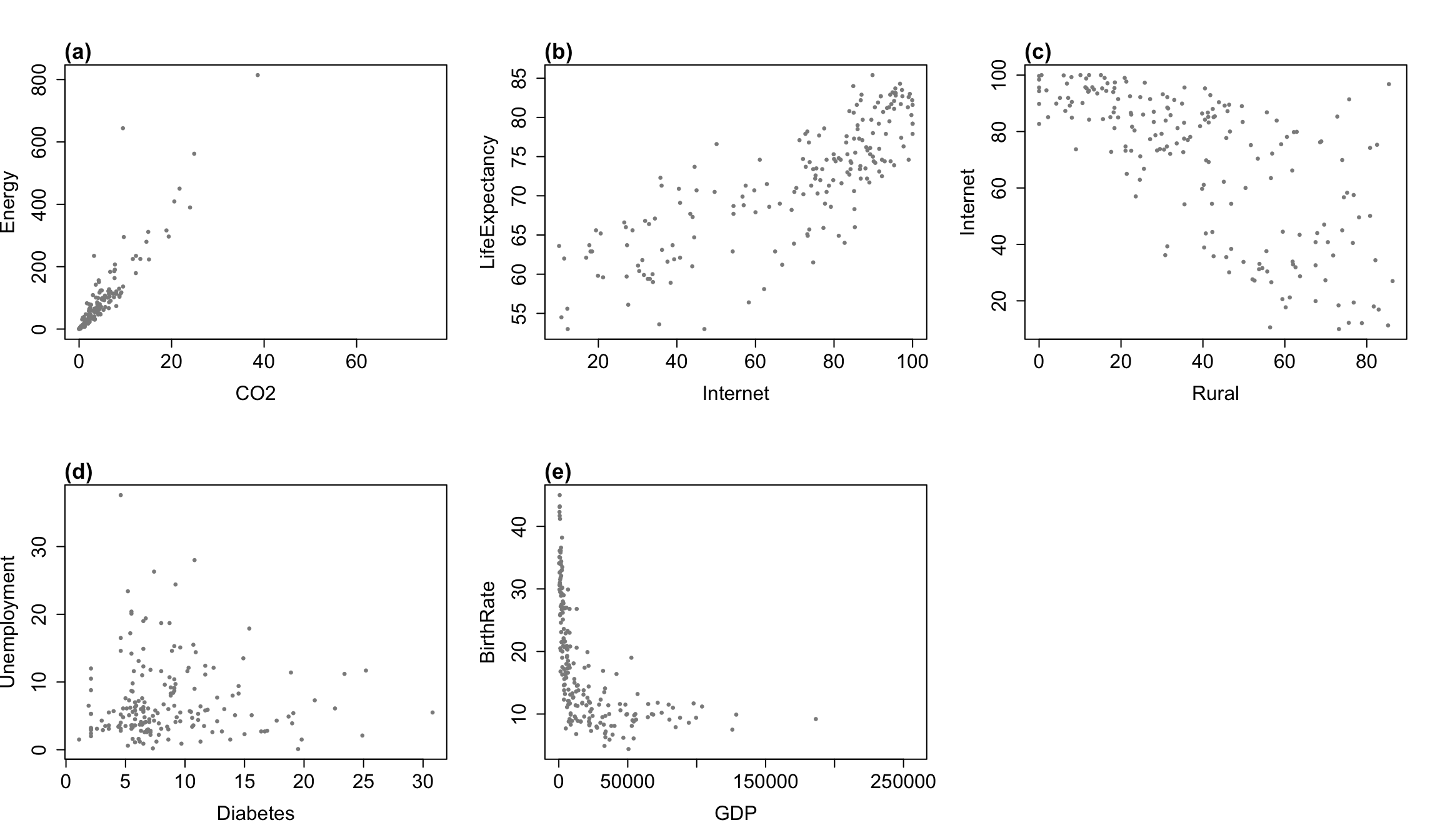
A scatterplot can visually display the linear relationship (positive or negative) between two numeric variables. The following graphs are based on the AllCountries dataset.

R code (optional)
data("AllCountries", package = "Lock5Data")

par(mfrow = c(2, 3))

plot(
  AllCountries$CO2, AllCountries$Energy,
  xlab = "CO2", ylab = "Energy", pch = 16, cex = 0.7, col = "gray55",
  cex.lab = 1.5, cex.axis = 1.5
)

mtext("(a)", side = 3, line = 0.2, adj = 0, cex = 1.1, font = 2)

plot(
  AllCountries$Internet, AllCountries$LifeExpectancy,
  xlab = "Internet", ylab = "LifeExpectancy", pch = 16, cex = 0.7, col = "gray55",
  cex.lab = 1.5, cex.axis = 1.5
)
mtext("(b)", side = 3, line = 0.2, adj = 0, cex = 1.1, font = 2)

plot(
  AllCountries$Rural, AllCountries$Internet,
  xlab = "Rural", ylab = "Internet", pch = 16, cex = 0.7, col = "gray55",
  cex.lab = 1.5, cex.axis = 1.5
)
mtext("(c)", side = 3, line = 0.2, adj = 0, cex = 1.1, font = 2)

plot(
  AllCountries$Diabetes, AllCountries$Unemployment,
  xlab = "Diabetes", ylab = "Unemployment", pch = 16, cex = 0.7, col = "gray55",
  cex.lab = 1.5, cex.axis = 1.5
)
mtext("(d)", side = 3, line = 0.2, adj = 0, cex = 1.1, font = 2)

plot(
  AllCountries$GDP, AllCountries$BirthRate,
  xlab = "GDP", ylab = "BirthRate", pch = 16, cex = 0.7, col = "gray55",
  cex.lab = 1.5, cex.axis = 1.5
)
mtext("(e)", side = 3, line = 0.2, adj = 0, cex = 1.1, font = 2)
Show plot descriptions
  • (a) CO2 and Energy: A strong positive linear relationship.
  • (b) Internet and LifeExpectancy: A strong positive linear relationship, but weaker than (a) since the dots are more scattered.
  • (c) Rural and Internet: A strong negative linear relationship.
  • (d) Diabetes and Unemployment: Essentially no linear relationship. The points do not show a consistent upward or downward linear trend.
  • (e) GDP and BirthRate: Some non-linear relationship, with the points not following a straight-line pattern.

Note: strength describes how closely the points follow a straight-line pattern; slope describes how steep the line is. A correlation near zero means little or no linear relationship; a nonlinear pattern could still be present.

Pearson Correlation Coefficient

The Pearson correlation coefficient, denoted by \(r\), is a statistic that measures the direction and strength of the linear relationship between two numeric variables.

  • Direction: positive or negative (based on the sign of \(r\))
  • Strength: Cohen scale
Absolute value of correlation Strength
\(0.50 \le |r| \le 1\) Strong
\(0.30 \le |r| < 0.50\) Moderate
\(0.10 \le |r| < 0.30\) Weak
\(|r| < 0.10\) Negligible

Notes

  • Any correlation coefficient is between \(-1\) and \(1\).
  • \(r\) can be strongly affected by outliers.
  • \(|r|\) (i.e. the magnitude of the correlation) is unchanged by a linear transformation of either variable, but the sign of \(r\) changes if exactly one variable is multiplied by a negative constant.
  • A steeper slope does not mean a stronger correlation.
  • \(r = 0\) only means no linear relationship, but a nonlinear relationship may still exist.

Example

Download the AllCountries dataset and open it in Jamovi. Note that this is a CSV (comma-separated values) file, which is the preferred format for many statistical projects.

One downside is that descriptions of the variables are not included within the CSV file itself, but you can refer to the AllCountries variable codebook. It is a standard practice to provide data and its codebook separately.

Based on the AllCountries dataset, is there a relationship between carbon dioxide emissions (CO2) and energy use (Energy)?

Show solution \(r = 0.913\). There is a strong, positive linear relationship between carbon dioxide emissions and energy use: countries with higher CO2 emissions tend to use more energy, on average.

Jamovi procedure: Analyses - Regression - Correlation Matrix - Put the two variables (CO2 and Energy in this example) into the Variables box - (optional) check Correlation matrix under Plot to generate a scatterplot.

Exercise

In the following bivariate relationship questions, support your answer with an appropriate statistic. If there is a linear relationship, describe its direction and strength using Cohen’s scale. Interpret your answer in context.

Use the AllCountries dataset for these questions.

  1. Is there a relationship between internet access (Internet) and life expectancy (LifeExpectancy)?

  2. Is there a relationship between the rural population percentage (Rural) and internet access (Internet)?

  3. Is there a relationship between diabetes prevalence (Diabetes) and unemployment (Unemployment)?

Show solution
  1. \(r = 0.812\). There is a strong, positive linear relationship between internet access and life expectancy. Countries with greater internet access tend to have higher life expectancy, on average.

  2. \(r = -0.690\). There is a strong, negative linear relationship between rural population percentage and internet access. Countries with a larger rural population percentage tend to have lower internet access, on average.

  3. \(r = 0.004\). There is a negligible linear relationship between diabetes prevalence and unemployment.

Correlation Coefficient: Other Cases

Pearson \(r\) is suitable for:

  • Scale + scale
  • Scale + dichotomous
  • Dichotomous + dichotomous

Spearman correlation coefficient, denoted by \(\rho\) (“rho”), is based on ranks and is suitable for:

  • Ordinal + ordinal
  • Ordinal + scale
  • Ordinal + dichotomous

Jamovi: Spearman \(\rho\) is obtained using the same procedure as Pearson \(r\), by selecting Spearman under the Correlation Coefficients option.

Correlation Coefficients: Summary

When using a correlation coefficient, report:

  • Direction

  • Strength

  • Interpretation in context

Exercise (cont’d)

4. (NELS) Describe the direction and strength, using Cohen’s scale, of the linear relationship between eighth-grade math achievement (achmat08) and teacher interest (tcherint).

5. (NELS) Is there an association between gender (gender; 0 = male, 1 = female) and eighth-grade math achievement (achmat08)?

6. (United States Colleges) Among schools in the United States Colleges dataset, is there an association between faculty size (faculty) and whether the school is a university (univ)?

7. (United States Colleges) Is there an association between affiliation (public; 0 = private, 1 = public) and institution type (univ; 0 = college, 1 = university)?

8. (United States Colleges) Is there an association between a school’s competitive rank (comp) and its student-faculty ratio (facratio)?

9. (United States Colleges) Is there an association between a school’s competitive rank (comp) and its faculty salary rank (facsal)?

10. (United States Colleges) Is there an association between a school’s competitive rank (comp) and affiliation (public)?

Show solution
  1. \(r = -0.203\). There is a weak, negative linear relationship between eighth-grade math achievement and teacher interest. The tcherint scale is coded so that lower values indicate greater teacher interest; students with higher math scores therefore tend to report greater teacher interest, on average.

  2. \(r = -0.132\). There is a weak, negative relationship between gender and eighth-grade math achievement. With gender coded 0 = male and 1 = female, female students tend to have slightly lower math scores than male students, on average.

  3. \(r = 0.499\). There is a moderate, positive relationship between faculty size and university status. Schools with larger faculties tend to be more likely to be universities.

  4. \(r = 0.501\). There is a strong, positive association between affiliation and institution type. Public schools tend to be universities, while private schools tend to be colleges.

  5. \(\rho = -0.343\). There is a moderate, negative linear relationship between competitive rank and student-faculty ratio. More competitive schools tend to have lower student-faculty ratios, on average.

  6. \(\rho = 0.594\). There is a strong, positive linear relationship between competitive rank and faculty salary rank. Schools with higher competitive-rank values tend to have higher faculty-salary-rank values.

  7. \(\rho = -0.234\). There is a weak, negative relationship between competitive rank and affiliation. Private schools tend to be more competitive, on average.

Bivariate Relationships Involving Nominal Variables

Introduction

If there is a nominal variable, we CANNOT! use a correlation coefficient to describe the bivariate relationship.

Intuitively, nominal variables are not ordered and do not have high or low values, so a correlation coefficient cannot be meaningfully interpreted.

A nominal variable is typically used as a grouping variable. In cases involving nominal variables, we compare different groups of people.

Compare medians:

  • Nominal + continuous
  • Nominal + ordinal

Compare percentages:

  • Nominal + dichotomous
  • Nominal + nominal

Compare medians

Nominal + Continuous

Example: (NELS dataset) is there a relationship between achmat8 (math achievement in 8th grade) and region?

Step 1: Identify the nominal grouping variable (region).

Step 2: Write down the groups as defined by the nominal variable:

  • Northeast
  • North Central
  • South
  • West

Step 3: Write down the MEDIANS of the other variable (achmat8) for each group.

Jamovi procedure: Explore -> Descriptives -> Variables -> achmat8 -> Split by -> region.

Step 4: If you detect relatively large differences in the medians, you can conclude that there is a relationship between region and achmat8. In your interpretation, describe the differences you see.

Show solution

Medians of achmat8 for each region:

  • Northeast: 58.6
  • North Central: 55.7
  • South: 54.9
  • West: 57.1

There is a relationship between region and achmat8: for instance, students from Northeast typically score higher than students from the South (medians: 58.6 vs 54.9).

Nominal + Ordinal

Example: (NELS dataset) is there a relationship between late12 (number of times late for school in 12th grade) and region? This is very similar to the previous example. Use the same steps to answer this question.

Show solution

Medians of late12 for each region:

  • Northeast: 1
  • North Central: 1
  • South: 1
  • West: 1

There is no relationship between region and late12. Regardless of region, students are typically late for school “1-2” times in 12th grade (median = 1 across all regions). Remember to check coding of the variable late12!

Additional notes

  • When asking if there is a “relationship” between region and achmat8, we want to know if there is a regional difference in terms of math achievement. Essentially, we are asking if the distribution of achmat8 differs across the four regions. The distribution can be different in many ways (think: location, spread, skewness). For instance, some regions might have more consistent performances (measure of spread); some regions might have more outliers (measure of shape). These are valid interpretations. For this class, however, we only require you to compare the medians (i.e., measure of location).

  • Can we also compare the means instead of the medians? Not in the second example, since late12 is an ordinal variable and the mean should not be used. In the first example (achmat8 - a continuous variable), the mean could be used IF there is no severe skewness and outliers, but the median is the more robust (“safer”) option.

Compare percentages

Nominal + Dichotomous

Example: (NELS dataset) is there a relationship between alcbinge (binged on alcohol ever) and region?

Option 1: Using region as a grouping variable:

  • Northeast:
  • North Central:
  • South:
  • West:

Option 2: Using alcbinge as a grouping variable:

  • Never binged:
  • Have binged:

Jamovi procedure

Refer to assignment 5 for more examples of contingency tables.

Analyses -> Frequencies -> Independent samples -> put one variable in Rows and the other in Columns. If the table looks hard to interpret, you can try switching row/column variables.

Percentages can be calcuated by checking relevant boxes under Cells - Percentages. I suggest that you only check “Row” percentages. You should never use “Total” percentages for bivariable relationships.

Visualizations can be obtained by checking Bar Plot under the Plots option. The “side by side” bar plot is sometimes referred to as a clustered bar graph.

Option 1: grouping by region

For each region, calculate the percent that have binged on alcohol:

  • Northeast:
  • North Central:
  • South:
  • West:

Conclusion:


Show solution
  • Northeast: 25.5% have binged on alcohol.
  • North Central: 23.8% have binged on alcohol.
  • South: 20.7% have binged on alcohol.
  • West: 15.1% have binged on alcohol.

There is a relationship between region and whether students have ever binged on alcohol. For instance, among students from the Northeast, 25.5% have binged on alcohol, while among students from the West, only 15.1% have binged on alcohol.

Option 2: grouping by alcbinge

  • Among people who have never binged on alcohol, what percentage comes from the South?
  • Among people who have binged on alcohol, what percentage comes from the South?

Conclusion:


Show solution
  • Among people who have never binged on alcohol, 30.4% are from the South.
  • Among people who have binged on alcohol, 28.7% are from the South.

(Not enough difference in percentages, so try a different region.)

  • Among people who have never binged on alcohol, 20.2% are from the West.
  • Among people who have binged on alcohol, 13.0% are from the West.

There is a relationship between region and whether students have ever binged on alcohol. For instance, among students who have binged, 13.0% are from the West; among students who have never binged, 20.2% are from the West.

In practice: choose a column and compare the “row” percentages in that column.

Nominal + Nominal

Example: Is there a relationship between schtyp8 (school type in 8th grade) and region? Calculate relevant percentages to support your answer. Make sure to interpret the percentages correctly.

Show solution

Option 1: Use region as the grouping variable.

  • Northeast: 67.9% attend public school.
  • North Central: 70.2% attend public school.
  • South: 76.0% attend public school.
  • West: 83.9% attend public school.

There is a relationship between region and school type: among students from the Northeast, 67.9% attend public school; among students from the West, 83.9% attend public school.

Option 2: Use schtyp8 as the grouping variable.

  • Public: 19.5% are from the Northeast.
  • Private, Religious: 26.7% are from the Northeast.
  • Private, Non-Religious: 25.0% are from the Northeast.

There is a relationship between region and school type: among students who went to public school, 19.5% are from the Northeast; among students who went to private, religious school, 26.7% are from the Northeast.

Common mistakes when interpreting contingency tables

Mistake 1: only describing ONE group to establish a bivariate relationship (i.e., if the percentages you “compare” add up to 100%, or they have the same denominator, you are probably making this mistake!)

Show example
  • “Among students from the NE, 67.9% went to public school vs 9.7% went to private, non-religious school.” This only describes the NE group and does not establish a relationship between region and school type. Maybe other regions also have about 67.9% of students attending public school and 9.7% attending private, non-religious school.

  • “Among violent adults, 98% drank milk as a kid vs 2% didn’t” - would this establish a relationship between violent behavior and milk consumption?

Mistake 2: incorrectly interpretating a percentage

Show example
  • How to interpret “67.9%”? You can say, among students from NE, 67.9% went to public school. You should NOT say “67.9% of students went to public school and are from the NE” (denominator would be 500). You should NOT say “67.9% of public school students are from NE” (denominator would be 370). Be precise about the denominator in your interpretation!

Mistake 3: draw a conclusion based on extremely imbalanced group sizes or small sample sizes

Show example
  • A company surveys workers about whether they had a workplace injury in the past year. One of the two overnight-shift workers reports an injury (50%), compared with 8 of 100 day-shift workers (8%). It would be misleading to conclude that overnight workers are much more likely to be injured based on only two overnight workers; one person’s response changes that group’s percentage by 50 percentage points. The company should collect data from more overnight workers and account for hours worked before comparing injury risk.

See StatChat 3 for discussions.

Additional examples

Contingency tables are useful for categorical variables (dichotomous, ordinal, nominal) in general.

Example 1: (United States Colleges) relationship between Affiliation (0 = private; 1 = public) and College or University (0 = college; 1 = university).

Example 2: (NELS) relationship between Urbanicity and edexpect (highest level of education expected)?

Show solution

Example 1.

Yes, there is a relationship between school affiliation and whether a school is a college or university. For example, among public schools, 93.5% are universities; among private schools, 43.4% are universities.

(OR) Yes, there is a relationship between school affiliation and institution type. Among universities, 56.6% are public, whereas among colleges, only 6.5% are public.

(OR) The correlation is \(r = 0.501\), indicating a moderate/strong, positive association. With public coded 1 and university coded 1, public schools tend to be universities, while private schools tend to be colleges.

Example 2.

Yes, there is a relationship between urbanicity and students’ educational expectations. For example, among students from rural areas, 40.1% expect a bachelor’s degree to be their highest degree, whereas among students from urban areas, 27.6% expect a bachelor’s degree to be their highest degree.

(OR) Yes, there is a relationship between urbanicity and students’ educational expectations. For example, among the 48 students who expect “less than college degree” to be their highest degree, 12.5% are from urban areas, whereas among the 103 students who expect Ph.D, MD, JD etc. to be their highest degree, 34% are from urban areas.

(OR) Spearman \(\rho\) can also be used if you consider urbanicity as an ordinal variable. \(\rho = -0.179\). There is a negative, weak relationship. Students from urban areas (LOW coding) tend to expect higher levels of education (HIGH coding), on average.

Review questions: fix and improve answers

Fix and improve: example 1

In the Combined Class Charities dataset, is there a relationship between Type (1=‘Animals’; 2=‘Environment’, 3=‘Human and civil rights’) and OS (Overall score)?

  • Since \(r = -0.028\), there is no relationship.

  • Since Type is nominal, there is no relationship.

Show solution

Should not use a correlation coefficient since Type is a nominal variable. The correct way is to compare the distributions (medians) of OS across different Type categories.

Fix and improve: example 2

In the NJ Restaurants dataset, is there a relationship between Type2 (1=‘French’, 2=‘American’, 3=‘Other’) and COST (cost of food)?

  • Since \(r = -0.382\), there is a negative, moderate relationship. French restaurants tend to have higher cost.

  • There is a relationship because the medians (40 and 2) are very different.

Show summary statistics
Statistic cost type2
N 40 40
Missing 0 0
Mean 39.6 2.10
Median 40.0 2.00
Standard deviation 7.83 0.810
Minimum 21.0 1
Maximum 59.0 3
Show solution

Should not use a correlation coefficient since Type2 is a nominal variable. The correct way is to compare the distributions (medians) of COST across different Type2 categories.

Fix and improve: example 3

In the NJ Restaurants dataset, is there a relationship between Type2 (1=‘French’, 2=‘American’, 3=‘Other’) and Sunday (does it open on Sunday, 0 = No, 1 = Yes)?

  • There is no relationship, since they have the same medians (2).
Show summary statistics

Descriptive statistics for type2, grouped by Sunday status:

Statistic sunday type2
N No 12
Yes 28
Missing No 0
Yes 0
Mean No 1.83
Yes 2.21
Median No 2.00
Yes 2.00
Standard deviation No 0.835
Yes 0.787
Minimum No 1
Yes 1
Maximum No 3
Yes 3
Show solution

Should not compare the medians of type2 since it is an ordinal variable. Should use a contingency table instead.

Fix and improve: example 4

In the United States Colleges dataset, is there a relationship between Competitiveness Ranking and College or University (0 = college, 1 = university)?

  • Since \(r = 0.099\), there is a positive, very weak relationship.

  • Colleges have lower competitiveness rank (mean = 3.02); universities have higher competitiveness rank (mean = 3.49).

Show summary statistics
Statistic univ comp
N College 92
University 152
Missing College 0
University 0
Mean College 3.02
University 3.49
Median College 2.00
University 2.50
Standard deviation College 2.26
University 2.34
Minimum College 0
University 0
Maximum College 8
University 8
Show solution

Should use Spearman \(\rho\) since Competitiveness Ranking is ordinal; comparing the distributions of comp between colleges and universities is also appropriate, but should use median instead of the mean, since comp is an ordinal variable.

Appendix

Choice of method summary

Bivariate relationships without any nominal variable:

  • Scale + scale: Pearson \(r\)
  • Scale + ordinal: Spearman \(\rho\)
  • Scale + dichotomous: Pearson \(r\) (the point-biserial correlation); compare the scale-variable distributions across groups
  • Ordinal + ordinal: Spearman \(\rho\); compare ordinal-response distributions across groups; contingency table
  • Ordinal + dichotomous: Spearman \(\rho\); compare ordinal-response distributions across groups; contingency table
  • Dichotomous + dichotomous: Pearson \(r\) (the phi coefficient); contingency table

Bivariate relationships with at least one nominal variable:

  • Nominal + scale/ordinal: compare outcome distributions across nominal groups
  • Nominal + dichotomous/nominal: compare category percentages using a contingency table

Visualizing relationships:

  • Scatterplots: two numerical variables
  • Side-by-side boxplots: one numerical variable and one categorical variable
  • Clustered bar graphs: two categorical variables
  • Contingency tables: two categorical variables