Chapter 2: Examining Univariate Distributions

STAT117: Introduction to Statistics

Introduction

  • Univariate distribution: describe ONE variable

  • Example: how would you describe the distribution of income in New Jersey? What about the distribution of education level?

  • Usually, a combination of tools can be used (e.g., statistics, table, visualizations)

  • The same information about a variable can be given by different tools

  • Choice of tools largely depends on the measurement type


Lecture notes and summary

To describe the distribution of income in New Jersey, we could report statistics such as the mean, median, and standard deviation, look at a frequency/percentile table, and/or plot a histogram or boxplot to visualize the shape, center, and spread (and check for skewness or outliers). Since income is continuous, tools like the mean, standard deviation, and histograms are appropriate.

To describe the distribution of education level, we could report a frequency table showing the count/percent of residents in each category (e.g., less than high school, high school, some college, bachelor’s, graduate degree) and display it with a bar chart. Since education level is ordinal (or sometimes treated as nominal), the median and percentiles make more sense than the mean, and cumulative percentages can be meaningful because the categories are ordered.

Frequency table - categorical variable

Lecture notes and summary

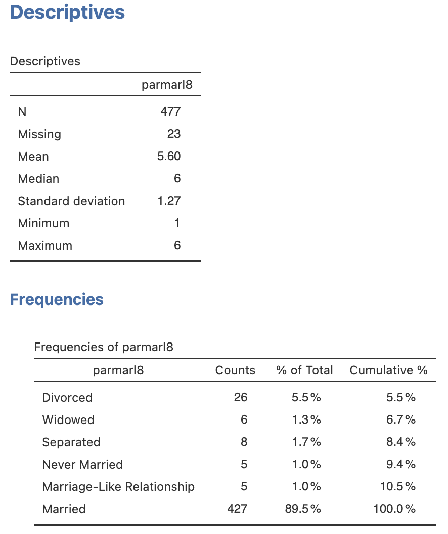
For the variable parmarl8 (Parents’ Marital Status in 8th grade):

  • % of Total example: \(5.5\% = 26 / 477\)

  • Cumulative % example: \(8.4\%\) for “Separated” = \(5.5\% + 1.3\% + 1.7\%\) (i.e., it is the sum of all percents up to that row)

  • Cumulative percent is NOT very useful in this case as it is a nominal variable

  • Should pay attention to how missing values are handled: in this case, by default, they are excluded from the percentage calculations
Frequency table - continuous variable

Lecture notes and summary

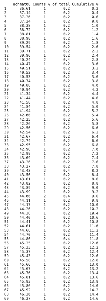
For the variable achmat08 (Math achievement in 8th grade):

  • % of Total example: \(0.2\% = 1 / 500\)

  • Cumulative % example 1: in row 30, a score of 42.54 has a cumulative percentage of \(6.2\%\), which means that \(6.2\%\) of students in the dataset scored 42.54 or lower

  • Cumulative % example 2: if I want to identify the bottom \(5\%\) of students, I would look for the row where the cumulative percentage reaches \(5\%\). The grade cutoff I’m looking for is 41.84

  • Counts and “%_of_total” columns are NOT very useful in this case as it is a continuous variable; most values have a count of 1 (i.e., unique scores); occasionally some values would have a count of 2 or more just due to coincidence
Percentile: intuitive examples

Lecture notes and summary

Percentiles compare one observation with a reference distribution. SAT reports show how a student’s score compares with scores from other test takers, while pediatric growth charts compare a child’s height or weight with measurements for children of the same age and sex.

Percentile and Percentile Rank

Kth percentile of a variable: a value that “beats” k% of the data
Family size frequency table

  • 25th percentile of family size:

  • 90th percentile of family size:

Percentile rank of a given value: % of data that are below the given value

  • Percentile rank of 4:

  • Percentile rank of 8:

Comparing percentile and percentile rank:

  • For example, after midterm 1, I can say “the 75th percentile of our class is 86.” What does that mean?

  • If your grade is 82, you could ask me what your percentile rank is. If the percentile rank of 82 is 62%, what does that mean?

Lecture notes and summary

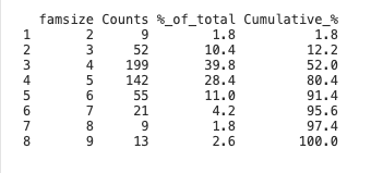
For the family-size table, the 25th percentile is 4: (at least) 25% of families have four or fewer members. The 90th percentile is 6: (at least)90% of families have six or fewer members.

The percentile rank of 4 is 52%, meaning 52% of families have fewer than four members. The percentile rank of 8 is 97.4%, meaning 97.4% of families have fewer than eight members.

The 75th percentile of 86 means that 75% of the class scored 86 or lower, and 25% scored above 86.

A percentile rank of 62% for a score of 82 means that 62% of class scores are below 82.

Percentile is a description of the distribution by identifying key positions (e.g., top position using 95th percentile; typical position using 50th percentile aka median).

Percentile rank is about an individual score; it describes the RANKING of that score in terms of the percentages.

Five Number Summary and IQR

Five Number Summary provides a quick snapshot of a continuous distribution:

  • Minimum (min):
  • First Quartile (Q1):
  • Second Quartile (Q2):
  • Third Quartile (Q3):
  • Maximum (max):

Interquartile Range (IQR)

Lecture notes and summary
  • Minimum: smallest observed value

  • \(Q_1\): 25th percentile

  • \(Q_2\): median, or 50th percentile

  • \(Q_3\): 75th percentile

  • Maximum: largest observed value

  • \(IQR = Q_3 - Q_1\)

  • Quartiles divide the data into four equal parts

  • IQR covers the middle 50% of the data

  • Range = max − min (covers all data); very affected by outliers

Boxplot

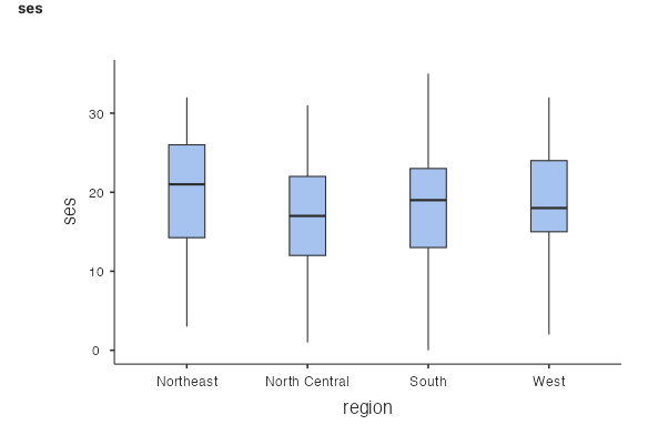
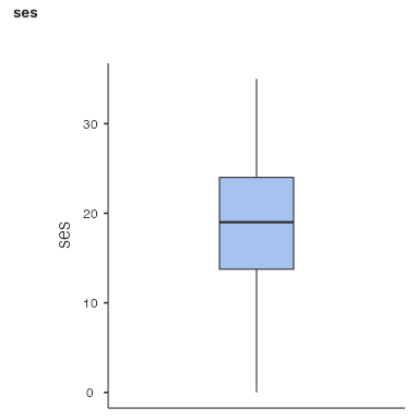
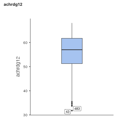
A boxplot is a visualization of the five number summary. It is made ONLY based on the minimum, Q1, median (Q2), Q3, and maximum.
Lecture notes and summary
  • Box in the middle: extends from Q1 to Q3, with a line at Q2 (median)
  • Whiskers: extend from Q1 down to the minimum, and from Q3 up to the maximum
  • Points: individual outliers (extreme values); the number on the outlier is the case number (e.g., row 43 is an outlier)

Boxplots can be useful for comparing distributions of a numeric variable across different groups

  • Example: Math Achievement by Geographic Region of School

  • The scale variable goes on the y-axis; the grouping variable goes on the x-axis

Bar Graph

Used for nominal/ordinal variables

Lecture notes and summary
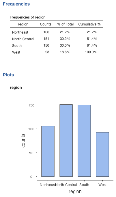
  • Bar graph: X-axis (categories) is not necessarily ordered
  • Width of bar: does not matter (unlike histograms)

In a bar graph for a nominal variable (like geographic region), the order of categories is arbitrary—you could rearrange them without changing the meaning. The width of each bar is just a visual feature; what matters is the height (frequency). This is different from histograms, where bar width represents a meaningful range of numeric values.

Histogram

Used for scale variables

Lecture notes and summary
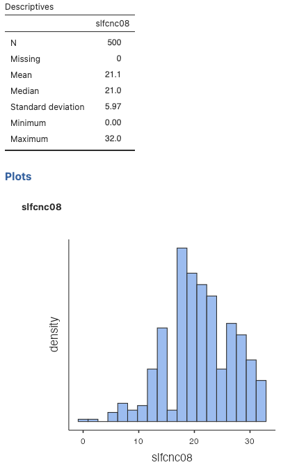
  • X-axis: ordered numeric values (e.g., math achievement)
  • Y-axis: frequency
  • Bar width: represents the range of values in each bin

A histogram is designed for numeric data. Its connected bars represent ordered intervals, allowing us to see the distribution’s overall shape, including its center, spread, skewness, and number of peaks.

Stem-and-Leaf

Let’s first take a look at A Japanese train timetable from 1985 (from Envisioning Information, Tufte)

A basic example:

data: 13 13 13 14 16 17 17 23 48 49 55 55 55 60 61 61 62 63 64 68

  The decimal point is 1 digit(s) to the right of the |

  1 | 3334677
  2 | 3
  3 | 
  4 | 89
  5 | 555
  6 | 0112348
Lecture notes and summary

In this example, stem 1 represents values from 10 to 19, stem 2 represents values from 20 to 29, and so forth. Each leaf represents the ones digit of an observation.

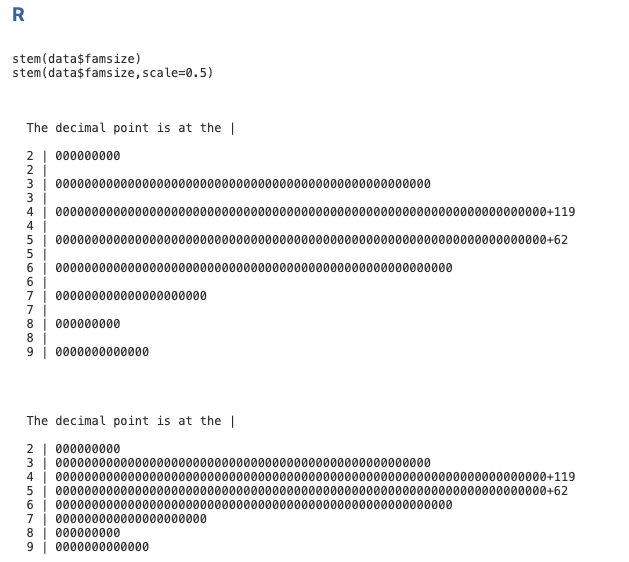
In a stem-and-leaf plot, the stem gives the leading digit(s) and each leaf represents a remaining digit. It displays the distribution’s overall shape while retaining individual observations.

Stem-and-Leaf

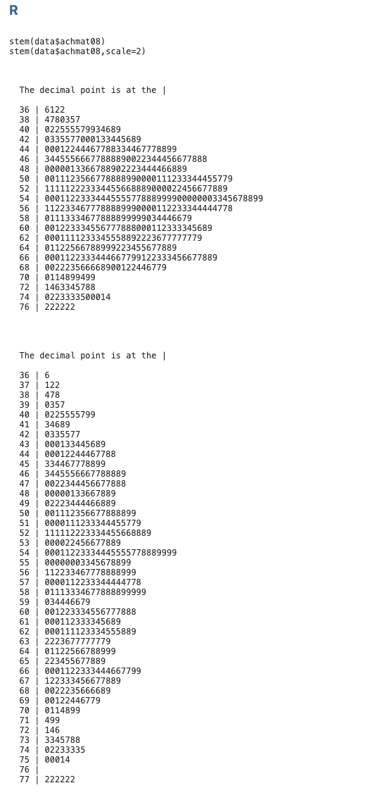
Stem-and-leaf plots are not very precise, and different software may use different rounding or grouping strategies, which can affect the appearance of the plot.
Family size
Math achievement in 8th grade

Lecture notes and summary

None.