Lecture 7: Bootstrapping

DATA 352/551: Modeling and Simulation

Review and introduction

Set-up

Material is based on The Incubation Period of Coronavirus Disease 2019 (COVID-19) From Publicly Reported Confirmed Cases: Estimation and Application, Lauer et. al., Annals of Internal Medicine, published online on March 10, 2020. Data and code are publically available.

nCoV_simple.csv: a simplified dataset that contains the incubation periods of \(50\) patients.

  • Create a vector called ncov10 based on the first \(10\) patients
ncov_simple <- read.csv('nCoV_simple.csv')
ncov10 <- round(head(ncov_simple$incubation, 10))
ncov10
 [1]  9 10  4  0  2  5 11  4  2  2

Introduction

Recall, a statistic is a function (i.e., a numeric summary) of data. A statistic is not the truth (i.e., parameter). We need to perform statistical inference.

summary(ncov10)
   Min. 1st Qu.  Median    Mean 3rd Qu.    Max. 
    0.0     2.0     4.0     4.9     8.0    11.0 

To make inference on the true average incubation period (\(\mu\)) based on the sample average (\(\bar{X} = 4.9\)), we need to understand the randomness of \(\bar{X}\) (i.e., its “sampling distribution”). Imagine two scenarios:

  1. Not much variation in \(\bar{X}\):
    • Confidence interval for \(\mu\):
    • Test the hypothesis that \(\mu \le 5\) days:
  2. A lot of variation in \(\bar{X}\):
    • Confidence interval for \(\mu\):
    • Test the hypothesis that \(\mu \le 5\) days:

Introduction

How do we know the sampling distribution of \(\bar{X}\)?

The sampling distribution of \(\bar{X}\) is well studied based on the Central Limit Theorem.

  • Shape:
  • Mean: \(\mu\) (population mean)
  • Standard Deviation (SD): \(\sigma/\sqrt{n}\) (where \(\sigma\) is the population SD)

Limitations:

  • CLT relies on a “large enough” sample size
  • CLT is only relevant when the statistic is the sample mean

Solution:

  • Bootstrapping does not rely on any modeling assumptions and can estimate the sampling distribution of any statistic!

Nonparametric Bootstrap

Introduction

  • “Pull yourself up by your bootstraps.”
  • Bootstrapping is a method that relies on resampling (with replacement) from the observed data.
    • Data: \(1, 1, 2, 3\)
    • Bootstrap sample:
    • Another bootstrap sample:
  • Often computationally intensive.
  • Developed by Bradley Efron in 1979.

Bootstrap samples

To get a bootstrap sample: resample the original data with replacement; sample size stays the same.

ncov10
 [1]  9 10  4  0  2  5 11  4  2  2
sample(ncov10, replace = TRUE)
 [1]  9  4  4  4  9 10  0 11  4  2
sample(ncov10, replace = TRUE)
 [1] 10  2 10 10  4  9  2  2 11  4
  • Repeat for many times and use the simulated means to study the randomness of the sample mean.

Exercise: Use the nCoV_simple dataset (incubation periods of \(50\) patients) to obtain \(B = 1000\) bootstrap samples; record the mean of each bootstrap sample in a vector called bootresult.

Show code
bootsize <- 1000
bootresult <- rep(NA, bootsize)
for (i in 1:bootsize) {
  bootresult[i] <- mean(sample(ncov_simple$incubation, replace = TRUE))
}

Inference using bootstrap samples

bootresult[1:30]
 [1] 3.8274 4.2132 4.1866 3.7988 3.9108 4.0790 4.2280 4.2412 4.2030 4.2524
[11] 4.0350 4.4518 3.5660 4.5024 3.7808 4.1226 4.1522 4.0546 3.6880 3.9010
[21] 4.1642 4.1008 4.2948 3.9846 4.8608 4.0856 4.3170 4.4646 3.4664 4.2500

Using the 1000 bootstrap samples, we can estimate the SD of \(\bar{X}\):

sd(bootresult)
[1] 0.3124195

In comparison, without using bootstrap, we can estimate the SD of \(\bar{X}\) with the formula: \(s/\sqrt{n}\)

sd(ncov_simple$incubation) / sqrt(50)
[1] 0.3309482

Inference using bootstrap samples

Show code
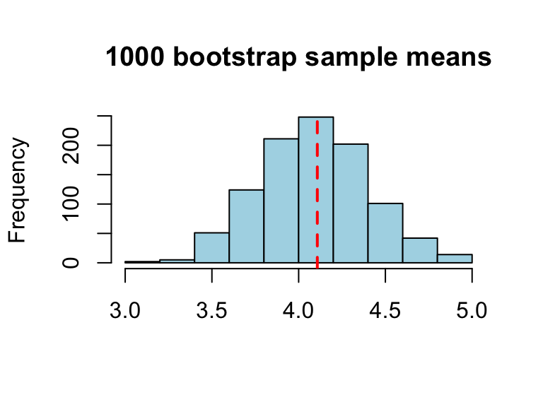
hist(bootresult, col='lightblue', main='1000 bootstrap sample means', xlab=NA)
abline(v = mean(ncov_simple$incubation), col='red', lty='dashed', lwd=2)

A 95% confidence interval of the mean incubation period

quantile(bootresult, probs = c(0.025, 0.975))
    2.5%    97.5% 
3.501790 4.740615 

Exercise: median

The median incubation period is often more of interest (why?) Compared to the mean, properties of the median are harder to calculate mathematically. Instead, we can use bootstrap to study these properties.

Exercise: use the nCoV_simple dataset

  1. Get the sample median of the dataset.
  2. Obtain \(B = 5000\) bootstrap samples; record the median of each bootstrap sample.
  3. Estimate the SD of the median. Does it have more variation or less variation compared to the mean?
  4. Obtain a 95% confidence interval for the median incubation period.
Show solution
#1
median(ncov_simple$incubation)
[1] 4
#2
bootsize <- 5000
bootresult <- rep(NA, bootsize)
for (i in 1:bootsize) {
  bootresult[i] <- median(sample(ncov_simple$incubation, replace = TRUE))
}

#3
sd(bootresult)
[1] 0.3952405
# more variation than the mean

#4
quantile(bootresult, probs = c(0.025, 0.975))
 2.5% 97.5% 
 2.92  4.50 

Limitations

The basic (nonparametric) bootstrap method does not work well in the following situations:

  • The original data are not independent.
  • The original data are not identically distributed.

Intuition: the resampling process ignores any dependence structure in the data;

  • We are studying the properties of a maximum or minimum.

Intuition: you would never exceed the maximum of the original data in a bootstrap sample, leading to underestimation of the variation of the maximum.

  • The underlying true distribution has a heavy tail.

Intuition: the resampling process tends to oversample extreme values in the original data.

Parametric Bootstrap

Introduction

Suppose we decide to fit a weibull distribution to the incubation period. We can then also estimate the probability that the incubation period is shorter than 14 days (call this \(\hat{p}\)).

library('MASS')
model1 <- fitdistr(ncov_simple$incubation, 'weibull', lower = 0)
pweibull(14, shape = model1$estimate[1], scale = model1$estimate[2])
[1] 0.9994694

What if we want to construct a confidence interval based on \(\hat{p}\)?

  • We would need to know the sampling distribution, or at least the variation, of \(\hat{p}\).

  • This can be difficult to derive if the model, and/or the parameter of interest, is complicated.

  • Instead, we will study the sampling distribution of \(\hat{p}\) using bootstrap.

Parametric bootstrap steps

  • Step 1: Fit the Weibull model (based on the original data) to obtain the plug-in distribution.

  • Step 2: Randomly sample another dataset (of the same sample size \(n=50\)) from the plug-in distribution.

bootdata <- rweibull(50, shape = model1$estimate[1], scale = model1$estimate[2])
  • Step 3: Re-fit the Weibull model with the new dataset.
modelboot <- fitdistr(bootdata, 'weibull', lower = 0)
  • Step 4: With the refitted model, record another value of \(\hat{p}\)
pweibull(14, shape = modelboot$estimate[1], scale = modelboot$estimate[2])
[1] 0.9992284
  • Step 5: Repeat steps 2, 3, and 4 to obtain many values of \(\hat{p}\). These values can be used to estimate the distribution of \(\hat{p}\)

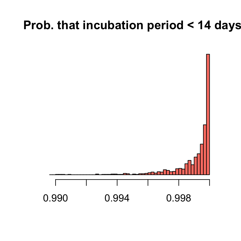
Exercise: Obtain \(1000\) values of \(\hat{p}\) using bootstrap. Plot a histogram of these values and construct a 95% confidence interval.

Show solution
# obtain plugin distribution
model1 <- fitdistr(ncov_simple$incubation, 'weibull', lower = 0)

# run bootstrap
bootsize <- 1000
result <- rep(NA, bootsize)
for (i in 1:bootsize) {
  bootdata <- rweibull(50, shape = model1$estimate[1], scale = model1$estimate[2])
  modelboot <- fitdistr(bootdata, 'weibull', lower = 0)
  result[i] <- pweibull(14, shape = modelboot$estimate[1], scale = modelboot$estimate[2])
}

hist(result,nclass=50,xlim=c(0.99,1),main='Prob. that incubation period < 14 days',
     yaxt='n',xlab=NA,col='salmon',ylab=NA)
quantile(result,c(0.025,0.975))
     2.5%     97.5% 
0.9950819 0.9999987 

Exercise: quantile estimates

  1. Fit the Weibull model to the incubation periods and estimate the 90th percentile of the incubation period (qweibull).
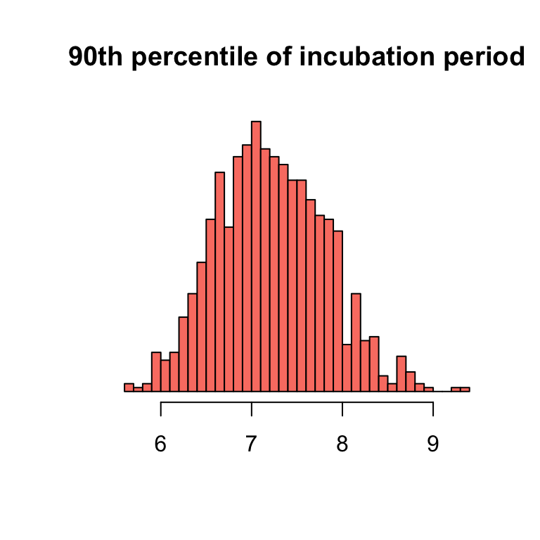
  2. Obtain \(B = 1000\) bootstrap samples from the plug-in distribution and estimate the SD of the 90th percentile.
  3. Obtain a 99% confidence interval for the 90th percentile of the incubation period.
Show solution
# obtain plugin distribution
model1 <- fitdistr(ncov_simple$incubation, 'weibull', lower = 0)
qweibull(0.9, shape = model1$estimate[1], scale = model1$estimate[2])
[1] 7.293084
# run bootstrap
bootsize <- 1000
result <- rep(NA, bootsize)
for (i in 1:bootsize) {
  bootdata <- rweibull(50, shape = model1$estimate[1], scale = model1$estimate[2])
  modelboot <- fitdistr(bootdata, 'weibull', lower = 0)
  result[i] <- qweibull(0.9, shape = modelboot$estimate[1], scale = modelboot$estimate[2])
}

hist(result,nclass=50,main='90th percentile of incubation period',
     yaxt='n',xlab=NA,col='salmon',ylab=NA)
quantile(result,c(0.025,0.975))
    2.5%    97.5% 
6.108560 8.397396