Lecture 4: Common Continuous Distributions

DATA 352/551: Modeling and Simulation

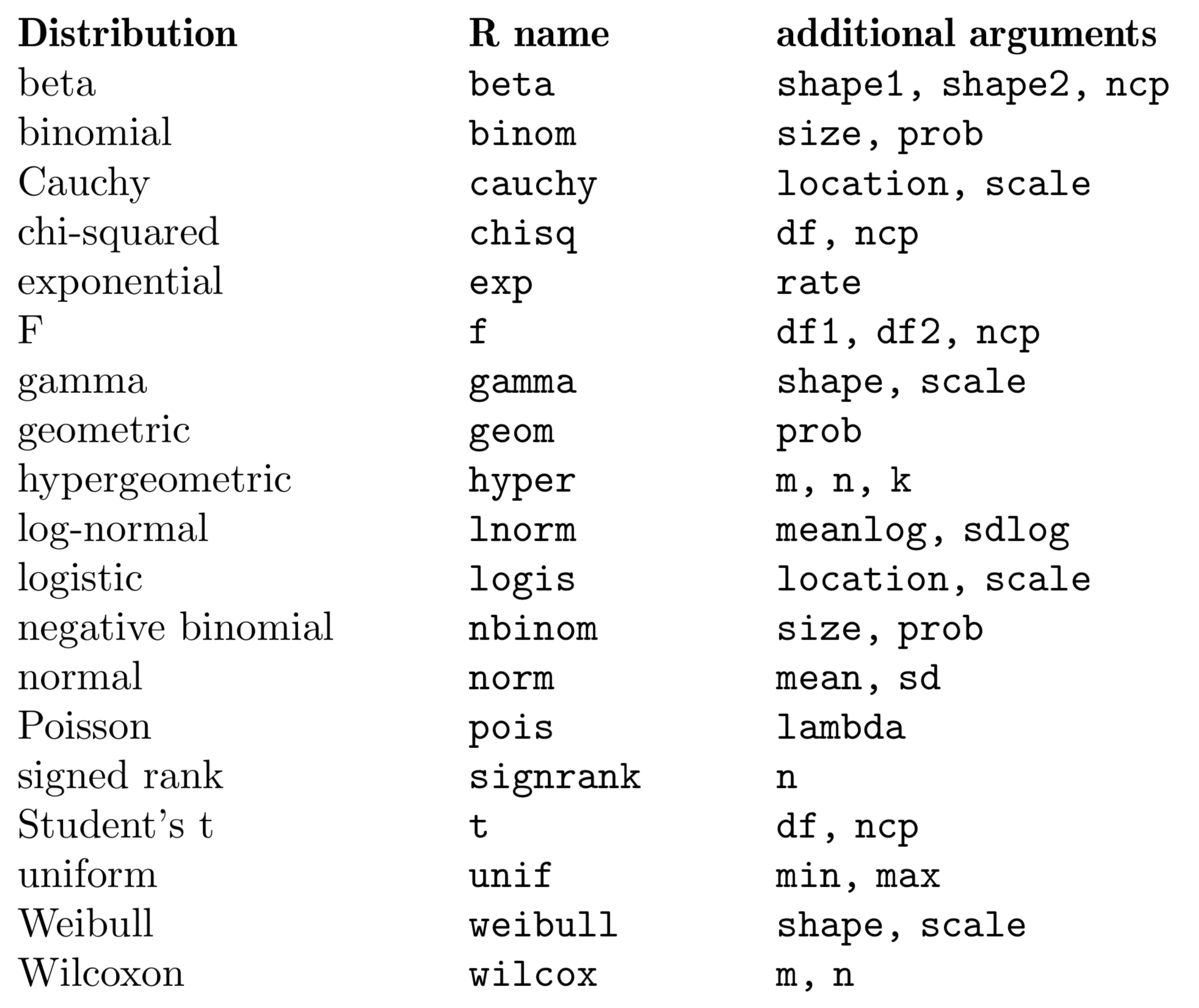
Distribution name reference in R

Continuous random variables

Recall, a random variable \(X\) is continuous if its sample space is continuous (and infinite). Can you think of some real life examples?


For discrete random variables, we calculate \(P(X=x)\) for each possible value. We cannot do the same with continuous random variables. Why?


Important property of a continuous random variable \(X\): \(P(X=x) = 0\) for any value \(x\). As a result:

  • For example: \(P(1 < X <3) = P(1 < X \le3) = P(1 \le X \le3)\).
  • Only makes sense to calculate \(P(X\in A)\) for some subset \(A \subset \mathbb{R}\).

Probability of continuous random variables

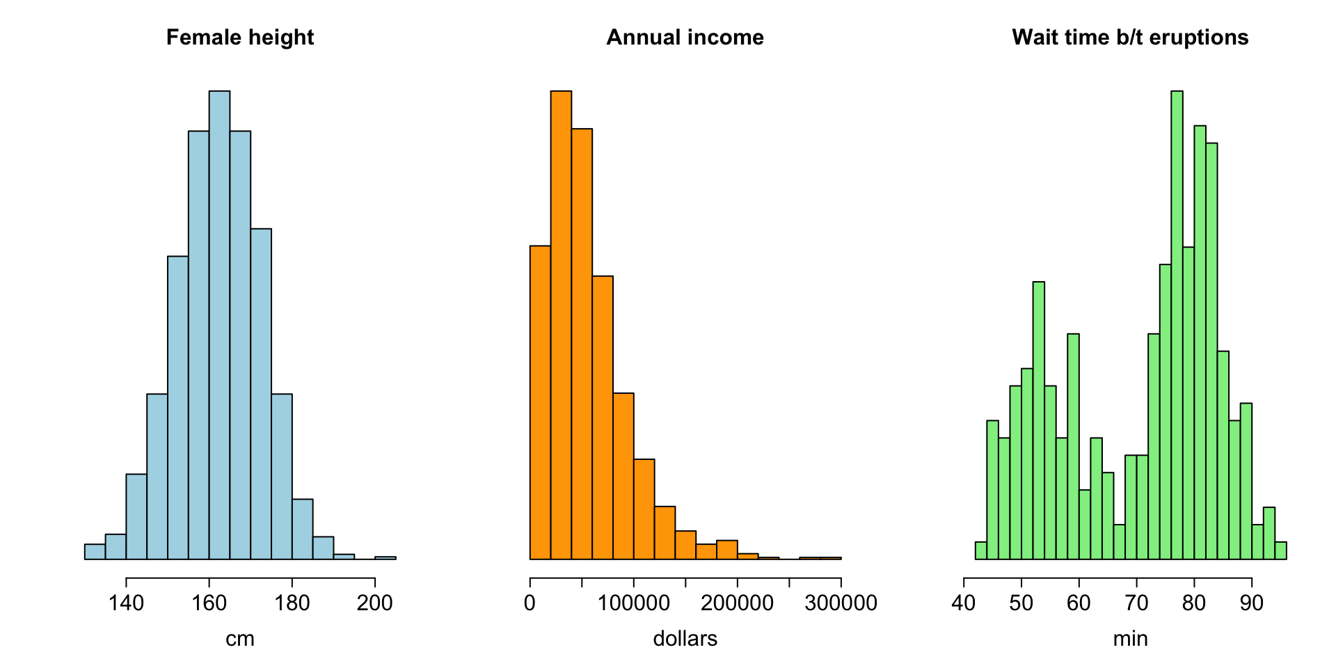
We can use histograms to visualize univariate, continuous distributions (the discrete equivalent is called a bar graph).

For the following continuous distributions, how would you calculate something like \(P( a<X<b)\)?

Show code
par(mfrow=c(1,3))
hist(rnorm(n=1000,mean=162,sd=10),freq=F,
     ylab=NA,
     xlab='cm',
     main='Female height',
     yaxt='n',
     col='lightblue',
     #border='blue',lty='dashed',
     nclass=20,
     cex.lab=1.5,
     cex.axis=1.5,
     cex.main=1.5)

hist(rgamma(n=1000,shape = 2,scale = 28000),freq=F,
     xlab='dollars',
     ylab=NA,
     main='Annual income',
     #cex.main=2,
     yaxt='n',
     col='orange',
     #border='blue',lty='dashed',
     nclass=20,
     cex.lab=1.5,
     cex.axis=1.5,
     cex.main=1.5)

hist(faithful$waiting,xlab='min', main='Wait time b/t eruptions',probability=T, 
     col='lightgreen',nclass=20, yaxt='n', ylab=NA,
     cex.lab=1.5,
     cex.axis=1.5,
     cex.main=1.5)

Density function

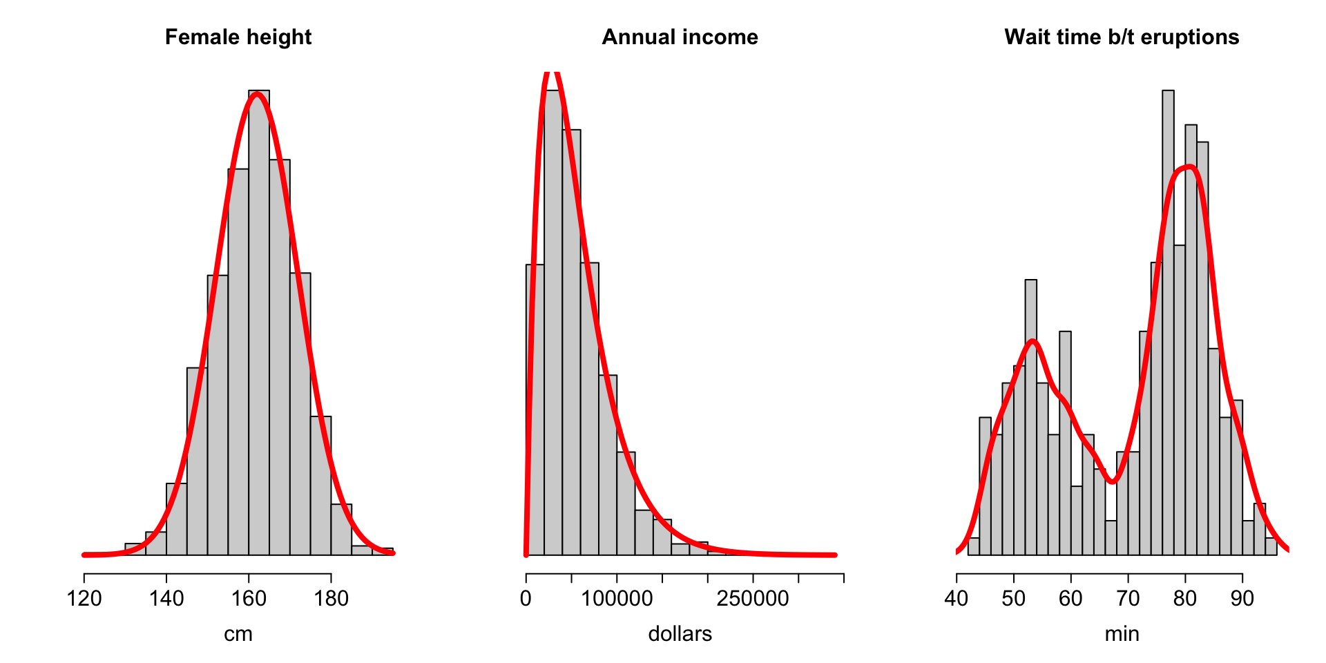
The probability mass function \(f(x)=P(X=x)\) cannot be defined for continuous random variables. Instead, we use something called the probability density function, defined as a function \(f(x)\) such that \(P(X\in A)=\int_A f(x) dx\).

Show code
par(mfrow=c(1,3))
hist(rnorm(n=1000,mean=162,sd=10),freq=F,
     ylab=NA,
     xlab='cm',
     main='Female height',
     yaxt='n',
     col='lightgrey',
     #border='blue',lty='dashed',
     nclass=20,
     cex.lab=1.5,
     cex.axis=1.5,
     cex.main=1.5)
curve(dnorm(x,mean=162,sd=10),add=T,col='red',lwd=4)

hist(rgamma(n=1000,shape = 2,scale = 28000),freq=F,
     xlab='dollars',
     ylab=NA,
     main='Annual income',
     #cex.main=2,
     yaxt='n',
     col='lightgrey',
     #border='blue',lty='dashed',
     nclass=20,
     cex.lab=1.5,
     cex.axis=1.5,
     cex.main=1.5)
curve(dgamma(x,shape = 2,scale=28000),add=T,col='red',lwd=4)

hist(faithful$waiting,xlab='min', main='Wait time b/t eruptions',probability=T, 
     col='lightgrey',nclass=20, yaxt='n', ylab=NA,
     cex.lab=1.5,
     cex.axis=1.5,
     cex.main=1.5)
dest = density(faithful$waiting,kernel = "gaussian",bw=2)
lines(dest, col = "red",lwd=4)
Density estimation

A small digression: density estimation is a very big topic in statistics. We’ll do a simple demo in R (R code: density(data, kernel = "Gaussian", bw = 5)).


For an arbitrary continuous density, calculating probabilities involves integration; R can handle common continuous distributions (i.e., their densities have certain functional forms, specified by given parameters); these are also used a lot in modeling.

Uniform

Uniform

Scenario: \(X\) is a random draw from the interval \((a,b)\)

Parameter: \(a\) and \(b\), end points of the range of \(X\)

Mean: \((a+b)/2\)

Probability:

  • dunif(2.3, min=0, max=3) does NOT give you probability!
  • punif(2.3, min=0, max=3) gives \(P(X\le2.3)\)

Simulation:

  • runif(1000, min=0, max=3)

Exponential

Exponential

Scenario: Exponential is often used to model Poisson waiting time: if the number of times an event occurs follows a Poisson distribution, then the waiting time between two events follows an exponential distribution.

Question: if you stand in front of a window and spot taxis at a constant rate of 12.5 taxis per hour, how long would you expect to wait for the next taxi?

Parameter: \(\lambda\) = rate of occurrence

Mean: \(1/\lambda\) = expected or average waiting time

Probability:

  • pexp(..., rate = ...)

Simulation:

  • rexp(1000, rate = ...)

Exercise

  1. Suppose speeding cars occur at a constant rate. A policeman stands at a certain location and catches one speeding car per 10 minutes, on average. What is the chance that he has to wait for less than 5 minutes to catch the next speeding car? More than 15 minutes? Between 5 and 10 minutes?


  1. Simulate from the above distribution; print out a few numbers and discuss what the numbers represent; plot a histogram to see its shape (note: the actual density function can be plotted by curve(dexp(x, rate = ...))).

Beta

Beta

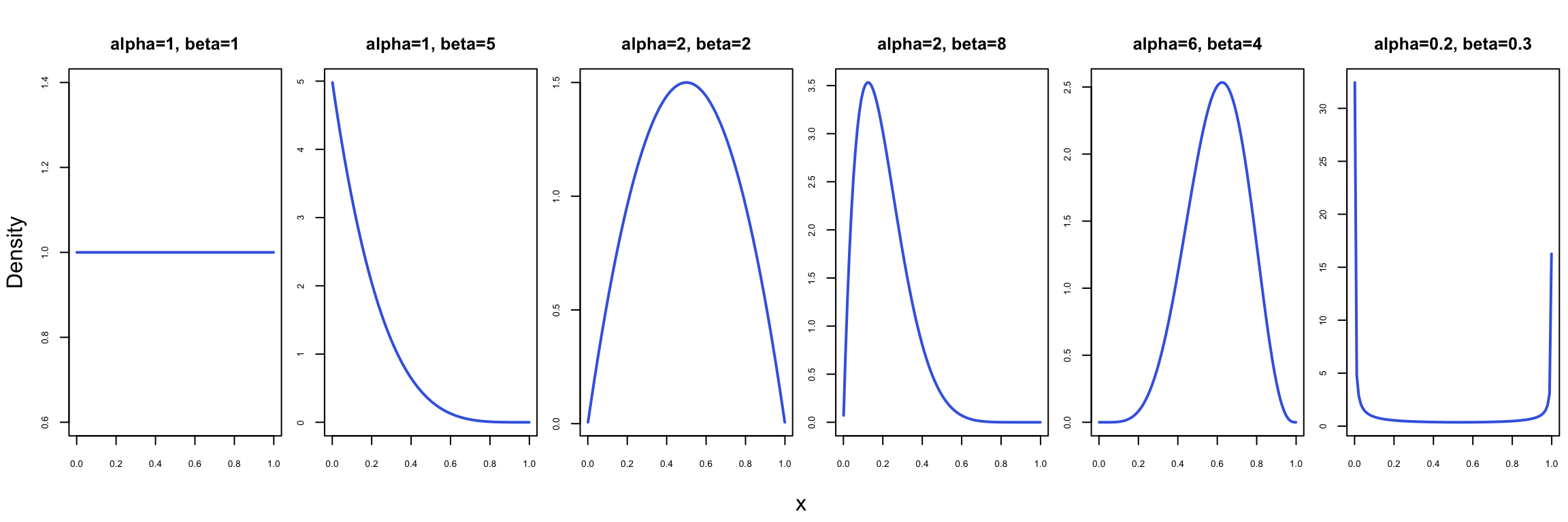
Scenario: Beta distribution has the range of \((0,1)\) and is often used to model percentages and probabilities, etc. (especially in Bayesian models as a prior distribution)

Parameter: \(\alpha\) = shape 1; \(\beta\) = shape 2

Show code
beta_shapes <- list(
     c(1, 1), c(1, 5), c(2, 2), c(2, 8), c(6, 4), c(0.2, 0.3)
)
beta_titles <- c(
     "alpha=1, beta=1", "alpha=1, beta=5", "alpha=2, beta=2",
     "alpha=2, beta=8", "alpha=6, beta=4", "alpha=0.2, beta=0.3"
)

par(mfrow = c(1, 6), mar = c(3, 2, 3, 0.5), oma = c(2, 2, 1, 0))
for (i in seq_along(beta_shapes)) {
     curve(
          dbeta(x, shape1 = beta_shapes[[i]][1], shape2 = beta_shapes[[i]][2]),
          from = 0.001, to = 0.999,
          col = "royalblue", lwd = 2,
          xlab = "", ylab = "", axes = TRUE, cex.axis = 0.65,
          main = beta_titles[i]
     )
}
mtext("x", side = 1, outer = TRUE, line = 0.5)
mtext("Density", side = 2, outer = TRUE, line = 0.5)

Mean: \(\alpha / (\alpha + \beta)\)

Probability:

  • pbeta(..., shape1 = ..., shape2 = ...)

Simulation:

  • rbeta(10000, shape1 = ..., shape2 = ...)

Normal

Normal

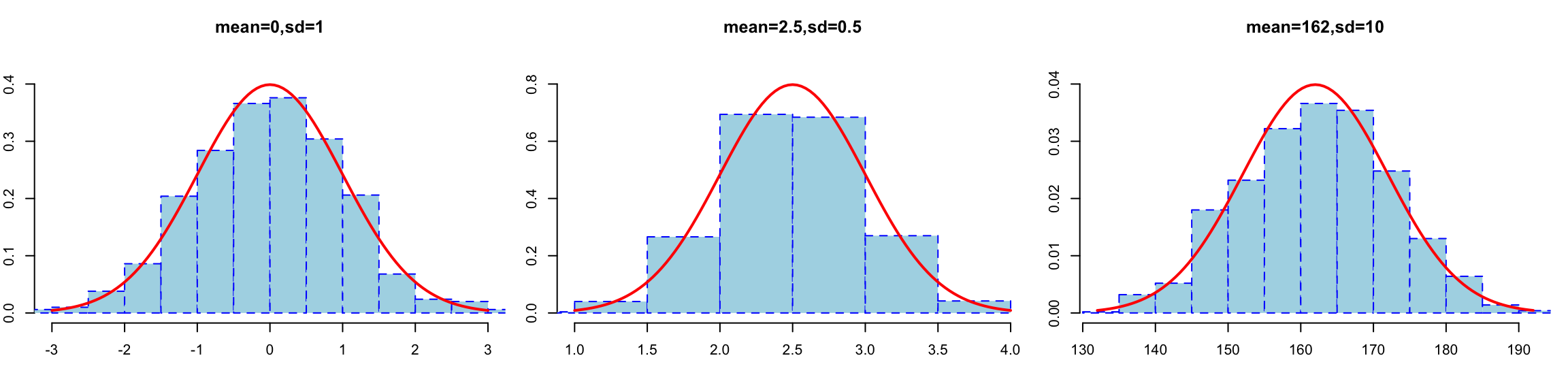
Scenario: Normal distribution is typically used to model the sum, or the average, of “identical and independent” random variables (e.g., distribution of the sample mean), due to the Central Limit Theorem.

Parameter: \(\mu\) = mean, \(\sigma\) = standard deviation

Show code
normal_means <- c(0, 2.5, 162)
normal_sds <- c(1, 0.5, 10)
normal_titles <- c("mean=0,sd=1", "mean=2.5,sd=0.5", "mean=162,sd=10")

par(mfrow = c(1, 3), mar = c(4, 2, 3, 1))
for (i in seq_along(normal_means)) {
  sample_values <- rnorm(1000, mean = normal_means[i], sd = normal_sds[i])
  hist(sample_values, probability = TRUE,
       main = normal_titles[i], xlab = "", ylab = "",
       col = "lightblue", border = "blue", lty = "dashed",
       ylim = c(0, 1.1 * dnorm(normal_means[i],
                              mean = normal_means[i], sd = normal_sds[i])),
       xlim = normal_means[i] + c(-3, 3) * normal_sds[i])
  curve(dnorm(x, mean = normal_means[i], sd = normal_sds[i]),
        add = TRUE, col = "red", lwd = 2)
}

Probability:

  • pnorm(..., mean = ..., sd = ...)

Simulation:

  • rnorm(10000, mean = ..., sd = ...)

Exercise

  1. A community survey uses a Beta(6, 2) model for the proportion of residents who support a proposal. What is the probability that support exceeds 80%?


  1. Exam scores are approximately normal with mean 80 and standard deviation 3. What proportion of students score between 75 and 85?


Notation for “distributed as”: %support ~ Beta(6, 2); score ~ Normal(mean = 80, sd = 3)

The Central Limit Theorem

Intuition: birthday example

If I pick a random student and ask their birth month, what number (between 1 and 12) would I get?

A. A small number (like 1 or 2)

B. A large number (like 11 or 12)

C. Around 6

D. No idea: any number is possible

Now, what if I ask a random sample of more than 1 students and calculate the average birth month? What would I get?

Simulation

  1. Suppose each of you is teaching a class with \(n=25\) students. Simulate \(25\) exam scores from uniform \((0,100)\) (try: plot a histogram of your simulated 25 exam scores; you should see a roughly uniform shape). Calculate the class average of your simulated class.

    Repeat for 10000 times, each time recording the class average. Plot a histogram of the 10000 simulated class averages. Estimate the mean and standard deviation (sd) of the class average?

  2. Repeat 1, but simulating \(25\) exam scores from normal with \(mean=80\) and \(sd=3\).

  3. Repeat 1, but simulating \(25\) exam scores from beta with \(shape1=6\) and \(shape2=2\).

Your results should show that, regardless of your starting distribution (uniform, normal, or beta), the simulated class AVERAGES are very “well-behaved”: the histogram of the 10000 simulated averages should look normal (symmetric bell-curve) in each case.

The Central Limit Theorem

Key result: if you have a random sample of \(n\) scores (these scores can be from ANY distribution!), then the sample average is random, and the randomness can be described by a normal distribution (for large \(n\)).

Why useful? CLT enables us to make statistical inference based on the sample mean. For instance, you might make a hypothesis that the exam scores follow a beta distribution with shape1=6 and shape2=2. To verify, you look at the average score of your 25 (randomly selected) students. CLT tells you what this average should look like under your hypothesis. If the observed average is “too extreme,” you might decide to reject the hypothesis.

Discussions

Important question: How large does \(n\) have to be for CLT to work well?

It depends on the shape of the population; if the population is very “not normal” (esp. long tail), \(n\) needs to be very large to overcome the “un-normalness.”

Supplementary material: